Download
1 / 54
540 likes | 666 Views
DoItQuick is a software company dedicated to assisting individuals with home finances, inventory management, and other tasks. After extensive analysis, it found that long-standing customers significantly outperform new customers in profitability. To enhance retention and maximize profit over a 20-year period, a consultant proposes a retention model based on customer loyalty and purchasing behavior. This report delineates the modeling of profits and the tools utilized to simulate customer lifetime value using the parameters of retention and discount rates.

E N D
Example 12.12 Marketing Models
Background Information • DoItQuick is software company that sells programs to individuals for keeping track of home finances, home inventory, and other common tasks. • The company has done extensive research into its costs and revenues, and it has discovered that new customers are much less profitable on an annual basis than long-standing customers. There are several reasons for this.
Background Information -- continued • Long-standing customers tend to require less in overhead costs, they tend to order more merchandise annually, and they help DoItQuick make money by referring new customers to the company’s products. • The company estimates that a customer who has been loyal for n years – that is has bought from the company for n consecutive years – contributes a normally distributed random amount of profit in the nth year that has mean and standard deviation as listed on the next slide.
Background Information -- continued • DoItQuick is interested in seeing how much profit a typical customer is worth over his or her years with the company. • This depends on the probability of retention. To model retention, let r(n) be the probability that a customer who has purchased for n consecutive years does not purchase the next year. • If this occurs, we assume that the customer switches loyalty and never purchases from DoItQuick again.
Background Information -- continued • A consultant has suggested to DoItQuick that a reasonable model of customer retention is to let r(1) = 1-p for some p between 0 and 1, and to use the equation r (n) = qr(n-1)for n>2, where q is a positive constant. • What does this model mean, and how can it and the data be used to simulate the nest personal value (NPV) of profit over a 20-year period from a typical customer who has made his or her first purchase from DoItQuick this year? Assume an interest rate of 10% for discounting.
Solution • The solution is broken into several parts. • First we will explain the consultant’s retention model. • Then we will fit curves to the profit data. • Finally, we will develop the simulation model and run it with @Risk.
Explaining the Retention Model • The consultant’s retention model makes sense. • First, p represents the probability that a customer who purchases this year for the first time will purchase again next year. • Then q is the fraction by which the probability of not remaining loyal changes year by year. • The company wants the r(n) values, the probabilities of losing customers, to be small, so it wants p to be large and q to be small. We will test several pairs of p and q when we run the simulation to see how these parameters affect the NPV of profit.
Finding the Data • We first use the ideas from Chapter 2 to fit equations to the means and standard deviations. • For each, we draw a scatterplot versus year, then superimpose an appropriate trendline with Excel’s Chart/Add Trendline menu item. • As shown in the figure, a logarithmic fit of the means looks good, whereas a linear fit of the standard deviation seems appropriate. • Therefore, in the simulation model we will estimate the mean and standard deviation of profit from a customer in her nth year with the company as –23.285 + 64.941ln(n) and 5.5515 + 1.3505n, respectively.
LOYALTY.XLS • The simulation model appears on the next slide. • This file contains the model.
Developing the Spreadsheet Model • The model can be developed with the following steps. • Inputs. Enter the inputs in the shaded cells. These include the parameter of the fitted equations for mean and standard deviation, the discount rate, and selected values of the retention parameters p and q. • Simulation index. We will use RISKSIMTABLE to run the simulation 12 times, once for each combination of p and q. To set up the model to do this, enter the formula RISKSIMTABLE(SimIndexes) in cell B11. Then obtain the corresponding values of p and q in cells B13 and B15 with the formulas =VLOOKUP(SimIndex,LookupTable,2) and VLOOKUP(SimIndex,LookupTable,3)
Developing the Spreadsheet Model -- continued • Profits. We want to simulate profits from a customer for as long as the customer remains loyal to the company. To do so, first calculate the appropriate means and standard deviations in columns B and C of the simulation section with the formulas =InterceptMean+SlopeMean*LN(A21) and =InterceptStdev+SlopeStdev*A21 in cells B21 and C21, and copy them down for all 20 years. Then generate the actual profits from this customer in column D as long as the customer remains loyal. Start by generating the first-year profit in cell D21 with the formula =RISKNORMAL(B21,C21) Then for succeeding years, enter the formula =IF(OR(F21=“Yes”,D21=“”),””,RISKNORMAL(B22,C22)) in cell D22 and copy it down. The OR condition checks whether the customer has discontinued buying from DoItQuick. If so, a blank is entered. Otherwise, a normally distributed profit is generated.
Developing the Spreadsheet Model -- continued • Probabilities of quitting. Calculate the probabilities of quitting in column E from the retention model. To do so, enter the formula =1-PrKeepBuying1 in cell E21. Then for succeeding years, enter the formula =IF(OR(F21=“Yes”,D21=“”),”” ,RetFactor*E21) in cell E22 and copy it down. • Quits? We keep track of the customer’s status in column F. First, enter the formula =IF(RAND( ) < E21,”Yes”,”No”) in cell F21. Then enter the formula =IF(OR(F21=“Yes”,D21=“”),””,IF(RAND( )<=E22, “Yes”, “No”)) in cell F22 and copy it down. This logic will produce several values of “No”, followed by a single “Yes” and then blanks.
Developing the Spreadsheet Model -- continued • Output cells. We will keep track of the NPV of profit and the number of years remaining loyal for this customer as @Risk outputs. Calculate these in cells B43 and B44 with the formulas =RISKOUTPUT( ) + NPV(DiscRate,Profits) and =RISKOUTPUT( )+COUNT(Profits). Note that the COUNT function counts nonblank cells only.
@Risk Results • We set the number of iterations to 1000 and the number of simulations to 12. • Selected summary results appear on the next slide. • For a change, we copied and pasted the @Risk results to the spreadsheet so that we could easily see how they vary with p and q. • The bar charts of the means clearly show how large values of p and small values of q are best for the company.
@Risk Results -- continued • By increasing the probability of keeping customers loyal, the company can make a big improvement in its bottom line.
Example 12.13 Consumer Preference Models with Correlated Values
Background Information • There are currently two brands of brownies on the market. • The Bisquake Company plans to enter the brownie market with one of two new brands. • Each of these existing brands and potential new brands is characterized by three attributes: sweetness (measured on a 1 to 10 scale), chewiness (measured on a 1 to 10 scale), and price per box. • These attributes are shown in this table.
Background Information -- continued • Each customer is assumed to choose one of these brands over the other on the basis of a weighted combination of the three attributes. • That is, each customer is assumed to calculate a score for each brand as Score = ws(Sweetness) + wx(Chewiness) + wp(Price)where the w’s are weights.
Background Information -- continued • Each customer’s weights are different, depending on how important sweetness, chewiness, and price are to the customer. However, we might expect these weights to be correlated. • For example, if a customer attaches a lot of importance to sweetness, she might also attach a large weight to chewiness; thus they would be positively correlated. • We assume that the population of customers assign normally distributed weights with the means and standard deviations shown in this table.
Background Information -- continued • We will also assume that the correlations between these weights are as given in the table below.
Background Information -- continued • Note that all correlations are positive, which implies that if a customer puts a large weight on one attribute, he will tend to put a large weight on the other two attributes. • Bisquake wants to use simulation to identify the new brand (from the two possibilities) that is likely to obtain the larger market share.
Simulation • A single iteration of this simulation will simulate the behavior of a single customer. That is, it will generate this customer’s weights, find the customer’s scores for each of these brands, and see whether the customer prefers new brand 1 or new brand 2 to the existing brands.
BROWNIE.XLS • This file provides the setup to develop the model seen on the next slide.
Developing the Spreadsheet Model • Inputs. Enter the inputs in the shaded ranges. These include the given means, standard deviations, and correlations for customers’ scores on the attributes. They also include the actual attributes of the two existing and two new brands. • Simulated weights. @Risk’s method of generating correlated random numbers is not very intuitive, but it is quite easy once you see how it works. We want the weights in the SimWeights range to be normally distributed with the means and standard deviations in the range B6:D7, but we also want them to be correlated. To accomplish this, generate the first weight (for sweetness) in cell B24 with the formula =RISKNORMAL(B6,B7,RISKCORRMAT (CorrMatrix,B23)) Then copy this to the range C24:D24 to generate the weights for the other two attributes.
Developing the Spreadsheet Model -- continued • It simply instructs @Risk to generate a normal random number but to correlate it with other potential random numbers, using the correlations in the first column of the CorrMatrix range. (It uses the first column because the second argument of RISKCORRMAT is 1.) For chewiness, this second argument is 2, and for price it is 3. This second argument essentially designates the position in the correlation matrix for the particular random value. • Scores for brands. Calculate this customer’s scores for the four brands in the range B27:B30 by entering the formula =SUMPRODUCT(SimWeights,B17:D17) in cell B27 and copying it to the range B28:B30. This formula weights the attributes of each brand with the customer’s weights.
Developing the Spreadsheet Model -- continued • Is either new brand chosen? One of the new brands will be chosen if its score is larger than the larger score of the two existing brands. Therefore, enter the formula =RISKOUTPUT( )+IF(B29>MAX(ExBrScores),1,0) in cell B33 to check whether new brand 1 is preferred to the exiting brands. Then copy it to cell B34 to do the same for new brand 2. • Summarize output cells. The @Risk output cells, B33 and B34, contain 1 or 0 depending on whether either new brand is preferred to existing brands. We want to determine the fraction of the time these will be 1. To do so, we can run the simulation for many iterations and calculate the means of the output cells. This is because the average of a sequence of 0’1 and 1’s is the fraction that are 1’s. We can calculate these fractions directly in the spreadsheet by entering the formula =RISKMEAN(B33) in cell B37 and copying it to the cell B38.
Using @Risk • We set the number of iterations to 1000 and the number of simulations to 1. • After running @Risk, we see from cells B37 and B38 that new brand 1 preferred to existing brands in 64.7% of the iterations, and new brand 2 is preferred to existing brands in 76.6% of the iterations. • Based on this information, new brand 2 appears to be the more promising brand for BisQuake to market.
@Risk Results • How do these results depend on the correlation structure we assumed earlier? • We note that because price weights are negative, the positive correlation between the sweetness (or chewiness) and price is less intuitive. It says that large weights on sweetness tend to go with “large” weights on price. But because price weights are negative, a “larger” weight on price means a less negative weight for price – for example –5 is “larger” than –8. So the positive correlation between sweetness and price really means that if a customer puts a lot of weight on sweetness, he cares less about price.
@Risk Results • For the sake of argument, suppose you think that the weights a customer assigns to the three attributes are probabilistically independent. • Then we should change the correlations in all cells of the correlations matrix to 0 and rerun the simulation. • When we did this, the values in cells B37 and B28 changed to 69.8% and 82.2%. • This is not a dramatic change, but it does show that correlations can make a difference.
Example 12.14 A Market Share Model
Background Information • Sweetness and IceT are the two dominant companies in the bottled iced tea market. • Each currently possess 49% of the total iced tea market, with three smaller companies splitting the remaining 2%. • At the beginning of any year, a random number of new small companies enter the iced tea market. • The actual number of new entries is assured to be Poisson distributed with mean 1.
Background Information -- continued • After the new entries enter the market, there is a random shift in market share among all competitors. • Essentially, all competitors lose a random percentage of their market share to other competitors. • We will assume that each of these percentages is triangularly distributed with the parameters given in the table on the next slide. • Therefore, the more small companies there are in the market, the more of its market share Sweetness will tend to lose to them.
Background Information -- continued • At the end of each year, each of the small companies has a 50% chance of exiting the ice tea market. • Each small company that exits will lose its market share to Sweetness or IceT. • The percentage of this marketshare that goes to Sweetness is triangularly distributed with parameters 40%, 50%, and 60%; the rest goes to IceT. • The dominant companies, Sweetness and IceT, want to use simulation to see how their market share is likely to change over the next 10 years.
Solution • At the beginning of the year we observe the market shares of Sweetness, IceT, and the small companies (combined). • Next, we simulate the number of new entrants. Then we simulate the shifts in market share during the year. • Next, we simulate the number of small companies that exit at the end of the year, and we simulate the market shares that go to Sweetness and IceT. • Finally, we tally the total market share at the end of the year for all competitors.
ICETEA.XLS • This file provides the setup to develop the model seen on the next two slides.
Developing the Model • The model can be formed with the following steps: • Inputs. Enter the inputs shown in shaded ranges. • Beginning market shares. For year 1 the beginning market shares are inputs. For example, find the beginning market share for Sweetness in cell B35 with the formula =B5. For every other year, the beginning market shares are the ending market shares from the previous year. For example, find the beginning market share for Sweetness in year 2 by entering the formula =B66 in cell C35. Then copy this to the range C35:K37 for all the competitors over the remaining years.
Developing the Model -- continued • Entries to the market. In year 1 find the number of small companies before entries, the number of new entries, and the number of small companies after entries by entering the formulas =B9, =RISKPOISSON(MeanEntries), and =SUM(B40:B41) in cells B40, B41, and B42, respectively. Note that the RISKPOISSON function, which takes a single argument, generates the number of new entrants in a single year. For year 2 the number of small companies before entries is the remaining number from year 1. Therefore, enter the formula =B58 in cell C40. Then copy the formulas in cells C40, B41 and B42 across the rows.
Developing the Model -- continued • Market shares lost during the year. Generate the percentage of its market share Sweetness loses to IceT and to the small companies (combined) in year 1 by entering the formulas =RISKTRIANG($B$24,$C$24,$D$24)*B35 and =RISKTRIANG($B$25,$C$25,$D$25)*B35*B42 in cells B46 and B47 and then copy these across rows 46 and 47. Next, enter similar formulas in rows 49, 50, 52 and 53 for market share lost by IceT and the small companies. For example, the formula in cell B53 is =RISKTRIANG($B$31,$C$31,$D$31)*B37.
Developing the Model -- continued • Exiters. Rows 56-59 contain information about small companies before and after exiting. To calculate this information, enter the formulas =SUM(B37, B47,B50)-SUM(B52:B53), =IF(B42>0,RISKBINOMIAL(B42,$B$13),0), =B42-B57, and =IF(B42>0,(B57/B42)*B56,0) in cells B56, B57, B58, B59. The copy these across rows 56-59. The formula in B56 simply tallies the market shares lost and gained for the small companies before exiting takes place. The formula in B57 uses the RISKBINOMIAL function to generate the number of small companies and the probability that any company exits. Finally, the formula in B59 finds the amount of market share possessed by the exiting companies under assumption that all small companies have an equal market share.
Developing the Model -- continued • Market share gained by exiters. The assumption of the model is that the market share of the exiters in row 63 is split randomly between Sweetness and IceT. To generate the split, enter the formula =RISKTRIANG($B$20,$C$20,$D$20)*B59 and =B59-B62 in cells B62 and B63. Then copy these across rows 62 and 63. • Year-end market shares. Calculate the year-end market shares of Sweetness, IceT, and the small companies (combined) by entering the formulas =SUM(B35,B49,B52,B62)-SUM(B46:B47),=SUM(B36,B46,B53,B63)-SUM(B49:B50), and =B56-B59 in cells B66, B67, and B68. Then copy these across rows 66-68. If you like, you can check that the year-end market shares sum to 100% for each year, as they should.
Developing the Model -- continued • @Risk outputs. We have not yet designated any cells as @Risk output cells. There are at least two possibilities. If we are interested in only the final market shares after 10 years, we should designate cells K66, K67, and K68 as output cells. • Alternatively, if we want to see how market shares move through time, we can specify whole ranges as output ranges. When you do this, the formulas change slightly. For example, the formula in cell B66 becomes =RISKOUTPUT(,”Sweetness”,1)+SUM(B35,B49,B52,B62)-SUM(B46:B47) to indicate that this is the first cell in the Sweetness output range.
@Risk Results • We set the number of iterations to 1000 and the number of simulations to 1. • After running @Risk, we obtain histograms of market share after 10 years. The histograms can be seen on the next two slides. • We see that the final IceT market share is essentially symmetric around its original value of 49%, although there is considerable variability. • In contrast, the final market share for the small companies has a good chance of being 0, although there is a small probability that it could be considerably larger – up to 8%, say.