Download
1 / 36
360 likes | 484 Views
Explore fundamental algorithm techniques including Divide and Conquer, Dynamic Programming, and Greedy Algorithms. This guide discusses the principles of each technique, with examples such as integer multiplication, closest pair of points, and efficient Fibonacci calculation. Understand how to analyze algorithms through recurrence relations and complexity. Learn about practical applications for optimization problems and how these strategies significantly reduce computational time. Whether you’re a novice or an experienced programmer, enhance your problem-solving skills with these powerful methods.

E N D
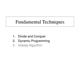
Fundamental Techniques Divide and Conquer Dynamic Programming Greedy Algorithm
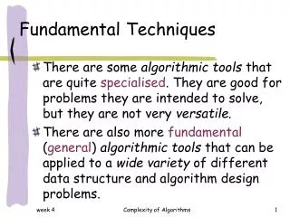
7 2 9 4 2 4 7 9 7 2 2 7 9 4 4 9 7 7 2 2 9 9 4 4 Divide-and-Conquer
Divide-and conquer is a general algorithm design paradigm: Divide: divide the input data S in two or more disjoint subsets S1, S2, … Recur: solve the subproblems recursively Conquer: combine the solutions for S1,S2, …, into a solution for S The base case for the recursion are subproblems of constant size Analysis can be done using recurrence equations Divide-and-Conquer
Computing integer power an • Brute force algorithm Algorithm power(a,n) value 1 for i 1 to n do value value a return value • Complexity: O(n)
Computing integer power an • Divide and Conquer algorithm Algorithm power(a,n) if (n = 1) return a partial power(a,floor(n/2)) if n mod 2 = 0 return partial partial else return partial partial a • Complexity: T(n) = T(n/2) + O(1) T(n) is O(log n)
Integer Multiplication • Multiply two n-digit integers I and J. ex: 61438521 94736407 • Complexity: O(n2)
subProblem1 subProblem3 subProblem4 subProblem2 Integer Multiplication • Divide : Split I and J into high-order and low-order digits. • ex: I = 61438521 is divided into Ih= 6143 and Il = 8521 • i.e.I = 6143 104 + 8521 • Conquer : define IJ by multiplying the parts and adding Complexity: T(n) = 4T(n/2) + n T(n) is O(n2).
subProblem1 subProblem3 subProblem1 subProblem2 subProblem2 Integer Multiplication • Improved Algorithm • Complexity: T(n) = 3T(n/2) + cn, • T(n) is O(nlog23), by the Master Theorem • Thus, T(n) is O(n1.585).
Closet Pair of Points • Given n-points find the 2 that are closest. y x
Distance Between Two Points • If the points are: (xi,yi) and (xj,yj) Distance = ((xi-xj)2+(yi- yj)2)
Closet Pair of Points • Brute-Force Strategy: • Compute distance between in each pair • Examine n(n-1)/2 pair of points • Determine the pair for which the distance is minimum • Complexity: O(n2)
L R Closet Pair of Points • Divide and Conquer Strategy. y x
Closet Pair of Points • Divide and Conquer Strategy. • Divide the point set to roughly two sub-sets L and R • Recursively Determine the Closest Pair of Points in L and in R. Let the distances bedL , dR • Determine the closest pair such that one is L and the other in R. Let the distances bedC • From the three closest pairs select the one with least distance.
Closet Pair of Points • Let = min(dL , dR) y x
2 Closet Pair of Points • For every point in the left region search for points in the right region in area 2 high Max 6 comparisons per point
Matrix Multiplication • Another well known problem: (see Section 5.2.3) • Brute force Algorithm: O(n3) • Divide and conquer algorithm; O(n2.81)
Dynamic Algorithm • Most difficult of the fundamental techniques. [Ref:Sahni, “Data Structure and Algorithms and Applications”] • Takes a problem that seems to require exponential time and produces polynomial-time algorithm to solve it. • The resulting algorithm is simple. Often requires a few lines of code.
Recursive Algorithms • Best when sub-problems are disjoint. • Example of Inefficient Recursive Algorithm: Fibonacci Number: F(n) = F(n-1) + F(n-2)
Recursive Algorithms function F(n) if n = 0 return 0 elseif n = 1 return 1 return F(n-1) + F(n-2) F(40) ~ 75 seconds F(70) ~ 4.4 years Complexity: T(n) 2T(n-1) + O(1) T(n) is O(2n) T(n) = 0.7236 * 1.618n- 1
Trace of Recursive Version F6 F5 F4 F2 F4 F3 F3 F1 F1 F1 F0 F2 F2 F3 F2 F1 F0 F1 F0 F1 F1 F0 F2 F1 F0 If we could store the list of all pre-computed values !!
Dynamic Programming • Find a recursive solution that involves solving the same problem many times. • Calculate bottom up and avoid recalculation
Efficient Version • Linear Time Iterative: Algorithm Fibonacci(n) Fn[0] 0 Fn[1] 1 for i 2 to n do Fn[i] Fn[i-1] + Fn[i-2] return Fn[n] Fibonacci(40) < microseconds Fibonacci(70) < microseconds
Efficient Version • Linear Time Iterative: Algorithm Fibonacci(n) Fn_1 1 Fn_2 0 Fn 1 for i 2 to n do Fn Fn_1 + Fn_2 Fn_2 Fn_1 Fn_1 Fn return Fn
Computing Binomial Coefficient (a+b)n = C(n,0)an +…+C(n,i)an-ibi +…C(n,n)bn Recursive Solution: C(n,0) = 1 for all n C(n,n) = 1 for all n C(n,k) = C(n-1,k-1) + C(n-1,k) for n>k>0
Computing Binomial Coefficient (a+b)n = C(n,0)an +…+C(n,i)an-ibi +…C(n,n)bn Dynamic Programming Solution: for i 0 to ndo C[n,0] 1 C[n,n] 1 for i 2 to n for j 1 to i-1 C[i,j] C[i-1,j-1] + C[i-1,j]
Dynamic Programming • Best used for solving optimization problems. • Optimization Problem defn: • Many solutions possible • Choose a solution that minimizes the cost
Review: Matrix Multiplication. C = A*B Aisd × eandBise × f O(d.f .e)time f B j e e A C d i i,j d f Matrix Chain-Products
Matrix Chain-Product: Compute A=A0*A1*…*An-1 Ai is di × di+1 Problem: How to parenthesize? Example B is 3 × 100 C is 100 × 5 D is 5 × 5 B*(C*D) takes 1500 + 2500 = 4000 ops (B*C)*D takes 1500 + 75 = 1575 ops Matrix Chain-Products
Matrix Chain-Product Alg.: Try all possible ways to parenthesize A=A0*A1*…*An`-1 Calculate number of ops for each one Pick the one that is best Running time: The number of paranthesizations is equal to the number of binary trees with n nodes This is exponential! It is called the Catalan number, and it is almost 4n. This is a terrible algorithm! An Enumeration Approach
Then total operations: A “Recursive” Approach • Find a recursive solution • Calculate bottom up and avoid recalculation • Let Ai is a di× di+1 matrix. • There has to be a final multiplication to arrive at the solution. • Say, the final multiply is at index i A0*…*Ai*Ai+1*…*An-1 = (A0*…*Ai)*(Ai+1*…*An-1). • Let N0,n-1 is number of operation for A0*…*Ai*Ai+1*…*An-1 N0,i for A0*…*Ai and Ni+1,n-1 for Ai+1*…*An-1
A “Recursive” Approach • Find a recursive solution • Calculate bottom up and avoid recalculation
A Dynamic Programming Algorithm • Find a recursive solution • Calculate bottom up and avoid recalculation • Running time: O(n3) AlgorithmmatrixChain(S): Input: sequence S of n matrices to be multiplied Output: number of operations in an optimal paranthization of S fori 0 ton-1 do Ni,i 0 forb 1 ton-1 do fori 0 ton-1-b do j i+b Ni,j fork itoj-1 do Ni,j min{Ni,j , Ni,k +Nk+1,j +di dk+1 dj+1} Length 1 are easy, so start with them Then do length 2,3,… sub-problems.
answer A Dynamic Programming Algorithm Visualization • The bottom-up construction fills in the N array by diagonals • Ni,j gets values from pervious entries in i-th row and j-th column • Filling in each entry in the N table takes O(n) time. • Total run time: O(n3) • Getting actual parenthesization can be done by remembering “k” for each N entry N n-1 … 0 1 2 j 0 1 … i n-1
Dynamic Programming • Is based on Principle of Optimality • Generally reduces the complexity of exponential problem to polynomial problem • Often computes data for all feasible solutions, but stores the data and reuses
When to Use Dynamic Programming? • Brute Force solution is prohibitively expensive • Problem must be divisible into multiple stages • Choices made at each stage include the choices made at previous stages.