Download
1 / 41
440 likes | 749 Views
The Aggregate Demand-Aggregate Supply (AD-AS) Model. Chapter 9. The Aggregate Demand Curve. The aggregate demand ( AD ) curve shows combinations of price levels and real income where the goods market is in equilibrium. The AD curve is an equilibrium curve. Aggregate production.

E N D
The Aggregate Demand-Aggregate Supply (AD-AS) Model Chapter 9
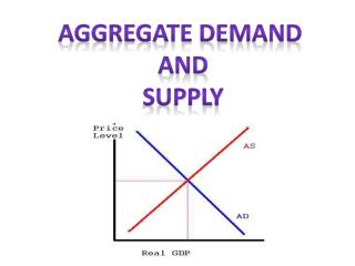
The Aggregate Demand Curve • The aggregate demand (AD) curve shows combinations of price levels and real income where the goods market is in equilibrium. • The AD curve is an equilibrium curve.
Aggregate production Derive the Aggregate Demand Curve Real expenditures AE1 (P1 < P0) B AE0 (P0) A Y0 Y1 0 Real income
Derive the Aggregate Demand Curve Price Level A P0 B P1 Aggregate Demand Real Output Y0 Y1
The Wealth Effect • Wealth effect – a fall in the price level will make the holders of money and other financial assets richer, so they buy more goods and services. • Most economists accept the logic of the wealth effect, however, they do not see the effect as strong.
The Interest Rate Effect • Interest rate effect – a lower price level raises real money balances, lowers the interest rate, and increases investment spending.
The International Effect • Internationaleffect – as the Canadian price level falls (assuming exchange rates do not change), net exports will rise. • Exports rise • Imports fall
The Multiplier Effect • Initial changes in expenditures set in motion a process in the economy that amplifies the initial effects. • Multiplier effect – the amplification of initial changes in expenditures.
Price level Wealth, interest rate, and international effects P0 Multiplier effect P1 Aggregate demand Y0 Y1 Ye Real output The AD Curve
Shifts in the AD Curve • Except for a change in the price level, anything that changes aggregate expenditures shifts the AD curve.
Shifts in the AD Curve • The main shift factors are: • Foreign income. • Exchange rate fluctuations. • Expectations about future output or prices. • The distribution of income. • Monetary and fiscal policies.
Monetary and Fiscal Policy • Macro policy – deliberate shifting of the AD curve. • Expansionary macro policy shifts the curve to the right. • Contractionary macro policy shifts it to the left.
Price level Initial effect Multiplier effect 100 200 P0 Change in total expenditures AD0 AD1 300 Real output Effect of a Shift Factor on the AD Curve
Short-Run Aggregate Supply Curve • The Short-run aggregate supply (SAS) curve shows how firms adjust the quantity of real output they will supply when the price level changes, holding all input prices fixed.
Price level Real output Short-Run Aggregate Supply Curve SAS
Shifts in the SAS Curve • The SAS curve shifts when a shift factor changes – other things are not constant: • Changes in costs of production. • Changes in expectations of inflation. • Productivity. • Excise and sales taxes. • Import prices.
Shifts in the SAS Curve • The net effect on prices is % change in the price level = % change in wages – % change in productivity
Price level Real output Shifts in the SAS Curve SAS1 Input prices increase SAS0
Long-Run Aggregate Supply Curve • The long run supply curve shows the amount of goods and services an economy can produce when both labour and capital are fully employed.
Long-Run Aggregate Supply Curve Long-run aggregate supply (LAS) Price level Real output
Potential Output and the LAS Curve • The position of the long-run aggregate supply curve is determined by potential output. • Potential output – the amount of goods and services an economy can produce when both labor and capital are fully employed.
Shifts in the LAS Curve • The LAS curve will shift whenever there is a changes in: • Capital. • Available resources. • Growth-compatible institutions. • Technology. • Entrepreneurship.
Price level F P1 Y0 Y1 Real output Short-Run Equilibrium:Shift in Aggregate Demand SAS E P0 AD1 AD0
Price level Real output Short-Run Equilibrium:Shift in Aggregate Supply SAS1 G P1 SAS0 E P0 AD Y1 Y0
LAS Price level H P1 E P0 Y0 Real output Long-Run Equilibrium:Shift in Aggregate Demand AD1 AD0
LAS Price level SAS E P0 AD Y0 Real output Long-Run Equilibrium
Recessionary Gap • A recessionary gap is the amount by which equilibrium output is below potential output.
Recessionary Gap • If the economy remains at this level for a long time, there would be an excess supply of factors of production. • Unemployment • Costs and wages would tend to fall. • As factor prices fall, the SAS curve will shift down to eliminate the recessionary gap.
LRAS Recessionary gap SAS0 SAS1 B Recessionary Gap Price level A P0 P1 AD Y0 Real output Y1
The Inflationary Gap • An inflationarygap occurs when equilibrium output is above potential. • Factor prices rise as firms compete for resources, causing the SAS curve to shift up. • The price level rises, and the inflationary gap is eliminated.
The Inflationary Gap LAS SAS2 D Price level P2 C SAS0 P0 AD Inflationary gap Y0 Y2 Real output (c)
Aggregate Demand Policy • Fiscal policy – the deliberate change in either government spending or taxes to stimulate or slow down the economy.
Aggregate Demand Policy • Expansionary fiscal policy is appropriate if aggregate income is too low. • The government can decrease taxes or increase government spending. • The deficit will increase. • The AD curve shifts to the right.
Expansionary Fiscal Policy LAS SAS0 Price level P1 P0 AD1 AD Y0 Y1 Real output (c)
Aggregate Demand Policy • Contractionary fiscal policy is appropriate if aggregate income is too high. • The government can increase taxes or decrease government spending. • The deficit will decrease. • The AD curve shifts to the left.
Contractionary Fiscal Policy LAS Price level SAS0 P0 AD P1 AD1 YP Y0 Real output (c)
Three Policy Ranges • An economy has three policy ranges where the effect of an expansion of AD on the price level will be different: • The Keynesian range. • The Classical range. • The intermediate range.
Price level Price/output path Real output Low potential High potential Three Ranges of the Economy Keynesian range Intermediate range Classical range Price level partially flexible Price level very flexible Price level fixed
Debates About Potential Output • Knowing potential output is crucial in knowing what policy to advocate. • According to real business cycle economists, the best estimate of potential output is the actual income in the economy.
Debates About Potential Output • Their Classical supply-side explanation is called real business cycle theory. • All changes in the economy result from real shifts—shifts in potential output—that reflect real causes, such as technological changes.
The Aggregate Demand-Aggregate Supply (AD-AS) Model End of Chapter 9