Download

1 / 45
450 likes | 571 Views
INTERANNUAL AND INTERDECADAL VARIABILITY OF THAILAND SUMMER MONSOON: DIAGNOSTIC AND FORECAST. NKRINTRA SINGHRATTNA CIVIL, ENVIRONMENTAL AND ARCHITECTURAL ENGINEERING DEPARTMENT UNIVERSITY OF COLORADO AT BOULDER 2003. MOTIVATION. THAILAND BACKGROUND

E N D
INTERANNUAL AND INTERDECADAL VARIABILITY OF THAILAND SUMMER MONSOON: DIAGNOSTIC AND FORECAST NKRINTRA SINGHRATTNA CIVIL, ENVIRONMENTAL AND ARCHITECTURAL ENGINEERING DEPARTMENT UNIVERSITY OF COLORADO AT BOULDER 2003
MOTIVATION THAILAND BACKGROUND • Location between 5-20 N latitudes and 97-106 E longitudes • Population ~ 61.2 million • Major occupation: agriculture (50%-60% of national economy) • Agriculture depends on precipitation and irrigation that is dependent on precipitation to store in reservoirs as well • “Precipitation” is crucial
MOTIVATION SEASON OF RAINFALL • 80%-90% of annual precipitation occurs during monsoon season (May-Oct) • Runoff is stored in reservoirs for use until the next year’s monsoon • Variability over inter-annual and decadal time scales • Need to understand this variability • All of these serve as “motivation” of this research
OUTLINE THAILAND HYDROCLIMATOLOGY 2. TRENDS 3. INTERANNUAL/INTERDECADAL VARIABILITY - RELATIONSHIP TO ENSO - PHYSICAL MECHANISM 4. PREDICTORS OF THAILAND RAINFALL 5. FORECASTING THAILAND MONSOON RAINFALL 6. CONCLUSIONS AND FUTURE WORK
DATA DETAILS • http://hydro.iis.u-tokyo.ac.jp/GAME-T • Thailand Meteorological Dept. • Six rainfall stations (r ~ 0.51) • Five temperature stations (r ~ 0.50) • Atmospheric circulation variables such as SLPs, SSTs and vector winds: NCEP/NCAR Re-analysis (www.cdc.noaa.gov)
DATA DETAILS • Correlation maps (CMAP and SATs) ensure their consistency • Thus, average rainfall ~ “rainfall index” average temperature ~ “temperature index”
MECHANISM OF CLIMATOLOGY • Spring (MAM) temperatures set up land-ocean gradient driving the summer monsoon • Summer monsoon (rainy season): Aug-Oct (ASO) • Little peak in May: Due to Northward movement of ITCZ • Enhanced MAM temperatures Enhanced ASO rainfall Decreasing monsoon seasonal (ASO) temperatures
MECHANISM OF CLIMATOLOGY • ITCZ northward movement: - Cover Thailand in May - Move to China in June - Southward move to cover Thailand again in August AM SON
TRENDS • Decreasing MAM temperature over decadal (-0.4 C) • Decreasing ASO rainfall (-180 mm) • Tend to cool land and atmosphere less Increasing ASO temperature • Trends after 1980: Increasing MAM temperature Increasing ASO rainfall (IPCC 2001 report) • Trends are part of global warming trends (IPCC 2001)
KEY QUESTION “What drives the interannual and interdecadal variability of Thailand summer monsoon?”
Schematic view of sea surface temperature and tropical rainfall in the the equatorial Pacific Ocean during normal, El Niño, and La Niña conditions .
FIRST INVESTIGATION • 21-yr moving window correlation with SOI index: Strong significant correlation only post-1980 • Spectral Coherence with SOI index
Correlation maps (pre- and post-1980) FIRST INVESTIGATION Pre-1980 Post-1980 SST SLP
To understand nonlinear relationship: Composite maps (pre- and post-1980) of high and low rainfall years (3 highest and lowest years) FURTHER INVESTIGATION Pre-1980 Post-1980 High Low
INSPIRED QUESTIONS “Why ENSO related post-1980 only?” “Is there change in ENSO after 1980?”
CONVECTION Pre-1980 Post-1980 correlation composite El Nino-La Nina Pre-1980 El Nino-La Nina Post-1980
ENSO INVESTIGATIONS Pre-1980 • Composite maps of SSTs: • Strong and eastward anomalies during post-1980 Post-1980
HYPOTHESIS “East Pacific centered ENSO reduces convections in Western Pacific regions (Thailand) while dateline centered ENSO decreases convections in Indian subcontinent” Pre-1980 Post-1980
COMPARISON WITH INDIAN MONSOON • To show changes in regional impacts of ENSO • 21-yr moving window correlation: Indian monsoon lose its correlation with ENSO around post-1980 • Thailand monsoon picks up correlation at the same time
CASE STUDIES 1997 2002 SST CMAP
SUMMARY (up to this point) • Strong relationship with ENSO during post-1980 • Indian monsoon shows weakening relationship with ENSO at the same time • Eastern Pacific centered ENSO (post-1980) contain descending branch over Western Pacific (included Thailand) • Dateline Pacific centered ENSO (pre-1980) contain descending branch over Indian subcontinent
REQUIREMENTS FOR GOOD PREDICTORS • Good relation with monsoon rainfall (post-1980) • Reasonable lead-time to forecast before monsoon season
CORRELATED WITH STANDARD INDICES • Significant correlations show 1-2 seasons lead-time
CORRELATION MAPS WITH LARGE-SCALE VARIABLES MAM AMJ MJJ SATs
CORRELATION MAPS WITH LARGE-SCALE VARIABLES MAM AMJ MJJ SLPs
CORRELATION MAPS WITH LARGE-SCALE VARIABLES MAM AMJ MJJ SSTs
TEMPORAL VARIABILITY OF PREDICTORS • 21-yr moving window correlation with three seasons (MAM, AMJ, MJJ) of all predictors • Indicate MJJ SLPs and MAM SSTs are the best predictors during post-1980 MAM AMJ MJJ
TRADITIONAL MODEL: LINEAR REGRESSION • Y = a * SLP + b * SST + e • e = residual: normal distribution with mean = 0, variance = 2 • Variable assumed normally distributed • Relationship among variables assumed linear relation • Drawbacks: • unable to capture non-Gaussian/nonlinear features • High order fits require large amounts of data • Not portable across data sets
NONPARAMETRIC MODEL: MODIFIED K-NN • Y = (SLPs, SSTs) + e • = local regression (residual: e are saved) • Capture any arbitrary: Linear or nonlinear • To forecast at any given “x*”, the mean forecast “y*” obtained by local regression (first step) • To generate ensemble forecasts: Resample residual (e) of neighbors “K” to “x*” by weighted assumption: • More weight to nearest neighbor, less weight to farther neighbor • Add residual to mean forecast “y*” • Be able to generate unseen values in historical data Resample “e” of neighbors E1 y* E2 E3 E4 x*
NONPARAMETRIC MODEL: MODIFIED K-NN • Number of neighbors for resampling residuals: “K” = (n-1) (n = # of variables) • Weighted function: W = 1/j (1/j) (j = 1 to “K”)
MODEL EVALUATION • Models are verified by cross validation • Data at given year is dropped out of the model • Model generates ensemble forecasts of the dropped year • Do for all years • Forecast will be evaluated by 3 criteria
CRITERIA OF MODEL EVALUATION • Correlation (r) between ensemble median and observed values: Rx,y = cov(x,y) ,cov(x,y) = (1/n)(xi-x)(yi-y) , higher;better x * y • Likelihood (LLH): Evaluates skill in capturing the PDFN [ Pf ]1/N t=1 LLH = 0 ~ no skill N [ Pc ] 1/N 1 – 3 ~ better to capture PDF t=1 • Rank probability skill score (RPSS): Evaluates skill in capturing categorical probability kij RPS = 1 [ ( Pn - dn)2] , RPSS = 1 – RPS (forecast) i=1n=1 n=1 RPS (standard) k –1 - < RPSS < +1 ; bad skill to perfect skill
MODEL SKILL R = 0.65 llh = 2.85 llh = 1.90 llh = 2.09 better skill: Higher r; LLH > 1; RPSS ~ +1 RPSS = 0.98 RPSS = 0.22 RPSS = 0.79 ALL YEARS WET YEARS DRY YEARS
SCATTER PLOTS Better forecasting in post-1980 R = 0.19 R = 0.21 R = 0.65 ALL YEARS PRE-1980 POST-1980
PDFs • PDF obtain exceedence probability for extreme events (wet: >700 mm and dry: <400 mm) show good skill (especially for wet scenarios)
CATEGORICAL PROBABILITY FORECAST • When cannot obtain large-scale variables • Use only forecasted categorical probability of ENSO • Quick and simple technique
PROBABILITY RELATIONSHIP • Conditional probability theorem: P(BA) = P(AB) P(A) • Total probability theorem: P(B(A1A2A3) = P(BA1)*P(A1)+P(BA2)*P(A2)+P(BA3)*P(A3)
CATEGORICAL PROBABILITY MODEL: ALGORITHM • Monsoon rainfall and standard index (SOI) are divided into 3 categorizes: Low, neutral, high (by 33rd and 66th percentile) • Estimate conditional probabilities • Forecasted categorical of SOI (P(SL),P(SN),P(SH)) are issued Estimate total categorical probability of monsoon rainfall (P(RL),P(RN),P(RH)) • To generate ensemble forecasts: Bootstrap historical data by total categorical probability
CASE STUDY Conditional Probability Forecasted Probability of SOI Total Categorical Probability of Rainfall
PDFs • Exceedence of extreme events (wet: >700 mm and dry: <400 mm) show considerate skill
CONCLUSIONS • Decreasing trend in MAM SATs and monsoon rainfall during 1950-2001 – slight increase during post 1980s • Thailand Monsoon rainfall shows strong relationship with ENSO in post-1980 while Indian monsoon lose its ENSO association in the same period • ENSO related Anomalies over eastern equatorial Pacific Walker circulation subsidence largely in the pacific region impacting south east Asia. Vice-versa for the Indian subcontinent. • Shifts in enso patterns post 1980 • Pre-monsoon SSTs and SLPs the tropical indian and pacific regions are identified as predictors of Thailand monsoon rainfall • Results from both statistical models show good skill at 1-4 months lead time • Significant implications to water (resource) management and planning
FUTURE WORK • Forecast improvement: Forecasts in this research is based on data during post-1980 only - Need to test this on data from other regions - Need to test this on earlier periods (e.g., pre 1950) on longer data sets • Streamflow forecasting : Obtain good quality streamflow data repeat analyses results directly impact reservoir operations and management • Causes for ENSO shifts: Area of active research (modeling and observational analysis) • Statistical-physical forecasting models: Combined statistical and physical watershed models can potentially improve the forecasts • Decision support system: to evaluate various decision options in light of the forecasts
ACKNOWLEDGEMENT • My sponsor: Public Works Department • Balaji Rajagopalan and all members of committee • Somkeit Apipattanavis • Katrina Grantz • Krishna Kumar