Quadratic-Solvability
Quadratic-Solvability. All you need is gap. Def : Quadratic-Solvability. An instance of Quadratic-Solvability ( QS [ ] ) is a system of quadratic-polynomials P 1 , …, P n over a field and variables y 1 , …, y m (where m n )

Quadratic-Solvability
E N D
Presentation Transcript
Quadratic-Solvability All you need is gap
Def: Quadratic-Solvability • An instance of Quadratic-Solvability ( QS[] ) is a system of quadratic-polynomials P1, …, Pn over a field and variables y1, …, ym (where m n) • Problem:to decide whether there exists a common root to all P1, …, Pn Thm[ GJ ]: QS[] is NP-hard (for any field )
Def: gap-QS[ D,, ] • An instance: a system of quadratic polynomials P1, …, Pn over a field , and variables y1, …, ym,where each Pidepends on at most D variables • Problem:distinguish between the following two cases: • yes: there exists a root common to all P1, …, Pn • no: any assignment to y1, …, yn zeros < fraction of P1, …, Pn
Reducing QS[] togap-QS[ n, , 2||-1 ] Thm[HPS]: gap-QS[ n, , 2||-1 ] is NP-hard As long as || ncfor some c>0 Proof: Given an instance P1, …, Pn of QS[] • set H so that |H| = ||½ • and d so that Hd = n • associate each point x Hd with a distinct quadratic-polynomial Px { P1, …, Pn } For any assignment A, denote by ƒA:Hd the function describing each Pi’s value on A Namely, ƒA(x), on every x Hd, equals Px[A]
Extension Consider now LDE[ƒA] namely, the low-degree-extension of ƒA to = d As seen in one of the early home assignments, LDE[ƒA]’s value on any x is a linear combination of A’s value on HdLDE[ƒA](x) = y Hd cxy · A(y) Let now Px, for every x ,bePx =y Hd cxy · Pythat is, a quadratic-polynomial being the corresponding linear combination of P1, …, Pn
The Resulting QS Instance {Px}x is a set of quadratic-polynomials, over the same variables y1, …, ymwhich for any assignment A satisfies the following: • If A zeros all Pi, then LDE [ƒA]is identically zero, and therefore A zeros Px for every x • In case LDE [ƒA] is not identically zero, like a good LDF it is almost nowhere zero, hence A zeros at most a very small (< r ||½)fraction of {Px}x
Our Goal • Thm[RS,DFKRS]:QS[ O(1), , 2/ ] is NP-hardas long as log|| logn for any constant < 1[ that is, the difference between Cook’s characterization of NP and PCP characterizations of NP (with constant number of variables each local-test depends on) boils down to the number of variables each polynomial accesses ]


