Chap 4-2. Frequency domain processing
Chap 4-2. Frequency domain processing. Jen-Chang Liu, 2006. Extend to 2-D DFT from 1-D. 2-D DFT: 1-D DFT in horizontal then vertical. Complex Quantities to Real Quantities. Useful representation. magnitude. phase. Power spectrum. 將影像用. 合成,其中. (u, v) 代表頻率. DFT. Real part.

Chap 4-2. Frequency domain processing
E N D
Presentation Transcript
Chap 4-2. Frequency domain processing Jen-Chang Liu, 2006
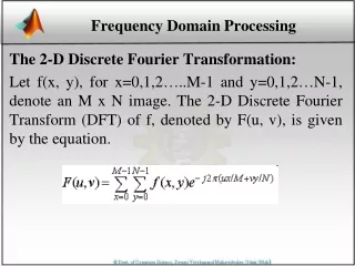
Extend to 2-D DFT from 1-D • 2-D DFT: 1-D DFT in horizontal then vertical
Complex Quantities to Real Quantities • Useful representation magnitude phase Power spectrum
將影像用 合成,其中 (u, v) 代表頻率 DFT Real part 2d DFT basis functions iDFT:
More DFT basis (real part) v (u,v)= (0,2) u (1,1) (1,0) (0,30) (1,30) (0,63) (30,30)
Example: reconstruction from DFT coefficients Zigzag scan …
Example: reconstruction from DFT coefficients http://www.ncnu.edu.tw/~jcliu/course/dip2005/lenaidft.m
imshow(log(abs(F)), []) Notes on showingDFT F(1,1)=7761921 F(1,127)=334.79+10i F=fft2(I); imshow(abs(F), []) Lena 256x256
Log transformations • s = c log(1+r) • Compress the dynamic range of images with large variation in pixel values
Periodicity and conjugate symmetry property of 2-D DFT M/2 M 0 N/2 N
Outline • Frequency domain operations • Smoothing Frequency Domain Filters • Sharpening Frequency Domain Filters • Homomorphic Filtering
mask coefficients X (product) output underlying neighborhood
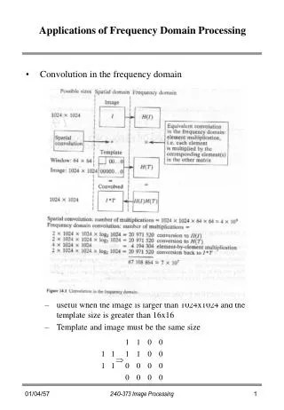
Convolution – 2-D case • 2d convolution 旋積 • Masking operation
Convolution theorem multiplication Frequency domain F H Fourier transform Fourier transform Time domain f:image h: filter or mask convolution
Filtering in the frequency domain fftshift
Outline • Frequency Domain Operations • Smoothing Frequency Domain Filters • Sharpening Frequency Domain Filters • Homomorphic Filtering
Smoothing frequency-domain filters • Design issue • G(u,v)=F(u,v) H(u,v) • Remove high freq. component (details, noise, …) • Ideal low-pass filter • Butterworth filter • Gaussian filter More smooth in the edge of cut-off frequency
Ideal low-pass filter • Sharp cut-off frequency where D(u,v) is the distance to the center freq.
Ideal low-pass filter (cont.) Cut-off freq.
Ideal low-pass filter (con.t) • ILPF can not be realized in electronic components, but can be implemented in a computer • Decision of cut-off freq.? • Measure the percentage of image power within the low freq. Total image power
ILPF: distribution of image power original Freq. 94.6 92 96.4 98 99.5
Ideal low-pass filtering a=92 D0=5 original a=94.6 D0=15 a=96.4 D0=30 a=98 D0=80 a=99.5 D0=230
Ringing effect
Effects of ideal low-pass filtering • Blurring and ringing ILPF: Freq. ILPF: spatial blurring F-1 ringing
Effects of ideal low-pass filtering (cont.) spatial spatial ILPF impulse
Butterworth low-pass filters H=0.5 when D(u,v)=D0
Order of butterworth filters Spatial domain filter of butterworth filters n=1 n=2 n=5 n=20 Ringing like Ideal LPF
Butterworth filters Order = 2 D0=5 original D0=15 D0=30 D0=80 D0=230
Gaussian low-pass filters Variance or cut-off freq. D(u,v)=D0 H = 0.607
Gaussian smoothing D0=5 original D0=15 D0=30 D0=80 D0=230
Practical applications: 1 GLPF, D0=80 444x508 斷點
Practical applications: 2 GLPF, D0=80 1028x732 GLPF, D0=100
Practical applications: 3 Scan line 588x600 GLPF, D0=30 GLPF, D0=10
Outline • Frequency Domain Operations • Smoothing Frequency Domain Filters • Sharpening Frequency Domain Filters • Homomorphic Filtering
Sharpening frequency-domain filters • Image details corresponds to high-frequency • Sharpening: high-pass filters • Hhp(u,v)=1-Hlp(u,v) • Ideal high-pass filters • Butterworth high-pass filters • Gaussian high-pass filters • Difference filters • Laplacian filters
Ideal HPF Butterworth HPF Gaussian HPF
Spatial-domain HPF Butterworth ideal Gaussian negative
Ideal high-pass filters original ringing D0=15 D0=30 D0=80
Butterworth high-pass filters n=2, D0=15 D0=30 D0=80
Gaussian high-pass filters D0=15 D0=30 D0=80
Laplacian frequency-domain filters • Spatial-domain Laplacian (2nd derivative) • Fourier transform
-(u2+v2) Laplacian frequency-domain filters Input f(x,y) F(u,v) F Laplacian -(u2+v2)F(u,v) F The Laplacian filter in the frequency domain is H(u,v) = -(u2+v2)
0 spatial H(u,v) = -(u2+v2) frequency
original Laplacian Scaled Laplacian original+ Laplacian
Outline • Frequency Domain Operations • Smoothing Frequency Domain Filters • Sharpening Frequency Domain Filters • Homomorphic Filtering
Image Formation Model Illumination source scene reflection eye
Homomorphic filtering • Image formation model • f(x,y)=i(x,y) r(x,y) reflectance: illumination: vary abruptly, particularly at the junctions of dissimilar objects Slow spatial variations
Homomorphic filtering • Product term • Log of product • f(x,y)=i(x,y) r(x,y) => ln f(x,y)=ln i(x,y)+ ln r(x,y) Separation of signal source:
Homomorphic filtering approach filtering lni(x,y) illumination lnr(x,y) reflection
How to identify the illumination and reflection? • Illumination -> low frequency • Reflection -> high frequency Example filter: sharpening Radius from the origin reflection illumination

