Frequency Domain Processing: 2-D DFT Fundamentals & Visualizations
Explore the fundamental principles and visualization techniques of 2-D Discrete Fourier Transformation. Learn about the Frequency Domain, Fourier Transform concept, and practical steps in DFT Filtering in MATLAB. Enhance your understanding with detailed instructions and code snippets. Discover how to calculate DFT, analyze Fourier spectrum, apply zero-padding, implement filtering, and obtain frequency domain filters from spatial filters efficiently.


Frequency Domain Processing: 2-D DFT Fundamentals & Visualizations
E N D
Presentation Transcript
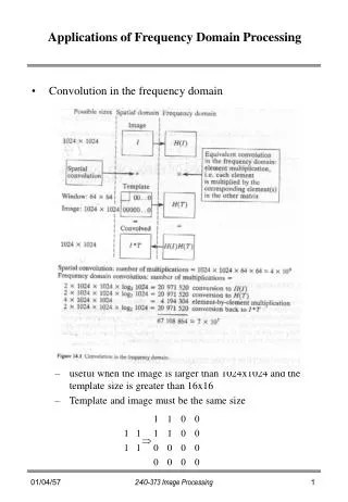
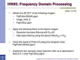
Frequency Domain Processing The 2-D Discrete Fourier Transformation: Let f(x, y), for x=0,1,2…..M-1 and y=0,1,2…N-1, denote an M x N image. The 2-D Discrete Fourier Transform (DFT) of f, denoted by F(u, v), is given by the equation.
Frequency Domain Processing The 2-D Discrete Fourier Transformation: For u=0,1,2….M-1 and v=0,1,2…N-1. The frequency domain is simply the coordinate system spanned by F(u, v) with u and v as (frequency) variables. The concept behind the Fourier transform is that any waveform that can be constructed using a sum of sine and cosine waves of different frequencies. The exponential in the above formula can be expanded into sines and cosines with the variables u and v determining these frequencies.
Frequency Domain Processing The 2-D Discrete Fourier Transformation:
Frequency Domain Processing Things to note about the discrete Fourier transform are the following: the value of the transform at the origin of the frequency domain, at F(0,0), is called the dc component F(0,0) is equal to MN times the average value of f(x,y) in MATLAB, F(0,0) is actually F(1,1) because array indices in MATLAB start at 1 rather than 0 the values of the Fourier transform are complex, meaning they have real and imaginary parts. The imaginary parts are represented by j, which is the square root of -1 we visually analyze a Fourier transform by computing a Fourier spectrum (the magnitude of F(u,v)) and display it as an image. the Fourier spectrum is symmetric about the origin the fast Fourier transform (FFT) is a fast algorithm for computing the discrete Fourier transform. MATLAB has three functions to compute the DFT:
Frequency Domain Processing Computing & Visualizing 2-D DFT in MATLAB: Create an image with a white rectangle and black background. f=zeros(30,30); f(5:24,13:17)=1; imshow(f)
Frequency Domain Processing Calculate the DFT. Notice how there are real and imaginary parts to F. You must use abs to compute the magnitude (square root of the sum of the squares of the real and imaginary parts). F=fft2(f,255,255); F2=abs(F); figure, imshow(F2,[])
Frequency Domain Processing To create a finer sampling of the Fourier transform, you can add zero padding to f when computing its DFT . F=fft2(f, 256,256); F2=abs(F); figure, imshow(F2, [])
Frequency Domain Processing The zero-frequency coefficient is displayed in the upper left hand corner. To display it in the center, you can use the function fftshift. F2=fftshift(F2); F2=abs(F2); figure,imshow(F2,[])
Frequency Domain Processing To brighten the display, you can use a log function. F2=log(1+F2); figure,imshow(F2,[])
Filtering in the Frequency Domain Basic Steps in DFT Filtering The following summarize the basic steps in DFT Filtering Obtain the padding parameters using function paddedsize: PQ=paddedsize(size(f)); Obtain the Fourier transform with padding:F=fft2(f, PQ(1), PQ(2)); Generate a filter function, H, of size PQ(1) x PQ(2).... Multiply the transform by the filter:G=H.*F; Obtain the real part of the inverse FFT of G:g=real(ifft2(G)); Crop the top, left rectangle to the original size:g=g(1:size(f, 1), 1:size(f, 2));
Frequency Domain Processing Basic Steps in DFT Filtering
f=zeros(50,50); • f(1:25,1:50)=1; • [M,N]=size(f); • F=fft2(f); • Sig=10; • H=lpfilter(‘gauss’,M,N,sig); • G=H.*F; • g=real(ifft2(G)); • Imshow(g,[])
Frequency Domain Processing Basic Steps in DFT Filtering >>f=zeros(50,50); >>f(1:25,1:50)=1; >>PQ=paddedsize(size(f)); >>Fp=fft2(f,PQ(1),PQ(2)); >>sig=10; >>Hp=lpfilter(‘gauss’,PQ(1),PQ(2),2*sig); >>Gp=Hp.*Fp; >>gp=real(ifft2(Gp)); >>gpc=gp(1:size(f,1),1:size(f,2)); >>imshow(gp, [ ])
Frequency Domain Processing Obtaining Frequency Domain Filters from Spatial Filters The filtering in spatial domain is more efficient computationally than frequency domain. One approach for generating a frequency domain filter, H, that corresponds to a given spatial filter, h, is to let H=fft2(h,PQ(1),PQ(2)) where the values of PQ depends on the size of the image we want to filter. The function freqz2 computes the frequency response of FIR (Finite Impulse Response) filters. H=freqz2(h, R, C) here R is num of rows and C is num cols R=PQ(1) C=PQ(2)
Frequency Domain Processing Obtaining Frequency Domain Filters from Spatial Filters