Download

1 / 1
10 likes | 137 Views
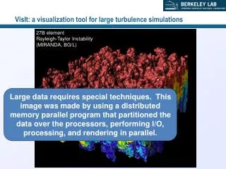
A UBK-space Visualization Tool for the Magnetosphere. Dipole B. Magnetopause. Dawn Tangency. Plasmapause. Separatrix. Dusk Tangency. Manish Mohan and Robert Sheldon UAH/NSSTC/MSFC 370 Sparkman Dr., Huntsville, AL 35805. Frames from the VRML interactive display.

E N D
A UBK-space Visualization Tool for the Magnetosphere Dipole B Magnetopause Dawn Tangency Plasmapause Separatrix Dusk Tangency Manish Mohan and Robert Sheldon UAH/NSSTC/MSFC 370 Sparkman Dr., Huntsville, AL 35805 Frames from the VRML interactive display. To better convey the interactive nature of the tool, we put some screenshots from a moving display. At the moment, the 3rd dimension has been modelled as pitchangle differences, or as E-field enhancements. This permits the direct comparison of dynamic changes, somewhat similar to holding 3 plots together over a desk lamp. However, for purposes of comparing, say plasmapause models to IMAGE data, one would prefer having the 3-D correspond to actual X,Y,Z pairs. This is a desirable modification of the C-code, which was written in 1991 before 3-D VRML was invented. ABSTRACT One of the stumbling blocks to understanding particle transport in the magnetosphere has been the difficulty to follow, track and model the motion of ions through the realistic magnetic and electric fields of the Earth. Under the weak assumption that the first two invariants remain conserved, Whipple [1978] found a coordinate transformation that makes all charged particles travel on straight lines in UBK-space. The transform permits the quantitative calculation of conservative phase space transport for all particles with E < ~100 MeV, especially ring current energies (Sheldon & Gaffey [1993]). Furthermore, as Sheldon & Eastman [1997] showed, this transform could extend the validity of diffusion models to realistic magnetospheres over the entire energy range. However, widespread usage of this transform has been limited by its non-intuitive use of UBK coordinates. We present a Virtual Reality Meta Language (VRML) interface to the calculation of UBK transforms, demonstrating its usefulness in describing both static features of the magnetosphere (plasmapause) as well as dynamic features (ring current injection & loss). The core software is written in C for speed, whereas the interface is composed of both Perl and VRML. The code is freely available, as is the web site, and intended for portability and modularity. Can we use UBK to analyze *real* data? Williams-Frank-Shelley Peak: When Don Williams was analyzing ISEE data he found a peak at the lower edge of his energy range. Comparing with the lower energy LEPEDEA instrument of Lou Frank, he found the same peak in the upper range. Adding in the composition instrument of Ed Shelley, he found a third confirmation of an odd peak in the data. Convinced it was real, he noted its peculiar pitch-angle distribution, and surmised that it might have something to do with locally accelerated particles due to waves. When Rob Sheldon analyzed this peak, he used UBK transforms calibrated for the Kp for each satellite pass. He then showed that the separatrix threading between the plasmapause proper and the “banana-orbit” portion, which is composed of the most deeply penetrating open drift trajectories from the plasmasheet uniquely identified the location of each of William’s peaks. What is VRML? The Virtual Reality Meta Language (VRML 1.0 and 97) is a programming language that permits the construction of 3-D worlds which can be drawn, manipulated, and navigated interactively. It uses a simple modelling language that is interpreted on a users local machine to keep the bandwidth to a minimum and the response optimally fast. It is implemented with browser plugins freely available on the web. ISEE orbit Kp=0.3, 3.5, 7.5 showing the shrinking of the plasmapause with increasing Volland-Stern electric field strength, using Maynard-Chen scaling.. (Kp=0 plasmapause is artifactually inflated). Why use VRML for UBK? VRML enables the user to examine 3-D (or multi-dimensional) data sets. A long-standing difficulty with magnetospheric physics is visualizing the trajectories of particles through the magnetosphere. Although UBK simplifies 2 of the dimensions, it takes some experience to build up the intuition. Seeing the particles in real-space, and observing how those surfaces transform in UBK space is essential in overcoming this barrier. With POLAR, IMAGE and soon-to-fly TWINS, we are now regularly retrieving 2-D projections of 3-D objects, it is vital to be able to rotate, project, analyze and visualize a 3-D distribution. This is what the UBK tool permits. (1) Solve complex models of B,U-fields for equipotential surfaces in UBK space (2) Transform back into Cartesian coordinates to visualize the projections in real space (3) Compare with data (4) Use the simplicity of UBK to modify boundary conditions, and iterate. Peak 1 Peak 2 Richmond 80 Ionospheric field Kp = 0.3, 3.5, 7.5 showing the opening up of the tangency surfaces with increasing Volland-Stern electric field, and the consequent better access of Plasmasheet particles into the magnetosphere. Acknowledgments This work has been partially funded by grant NASA/OSS GC 153274 NGD among others, and represents 11 years of development on UBK, with the contributions of 3 graduate students and 3 undergraduates. I especially want to thank Carl McIlwain and Elden Whipple who graciously got me started on this project. How Simple is it to find the Plasmapause in UBK? In UBK-space, the particles travel on straight paths with a slope proportional to the energy. Those that intersect a green tangency line “bounce” and reverse direction. If they intersect the red magnetopause, they are lost from the system. So the recipe for finding the plasmapause is simple: it’s the highest horizontal line that is trapped between green curves. (If one filled in the green curves with water, it’s the highest level the pond would reach.) We mark this surface with a blue line, and then map back into real space to see the effect. How can one use this UBK visualization tool? Glad you asked. It is freely available in beta-test source code. Presently the tool is written in C, and has a Perl wrapper that enables it to run with a WWW interface that generates HTML and VRML output for interactive viewing. The (somewhat buggy) package can be found at http : // cspar181.uah.edu/UBK/where it is being actively improved. Here are some screenshots of the interface as it presently stands. CONCLUSIONS UBK-space transformations have the power to solve the hoary problem of magnetospheric imaging, if only one can overcome the barrier of the non-intuitive UBK space. The use of VRML with an interactive graphical user interface is potentially capable of educating the intuition via the simulation of reality. As the sophistication of this tool increases, we hope that it will prove instrumental in the interpretation of graphical data sets returned by satellites such as POLAR and IMAGE. Community interest and feedback is encouraged by making the source code readily available and maintaining a WWW interface to the code. All code is in the public domain, much of it platform independent, permitting the installation of the entire WWW package on UNIX workstations. The graphics on this poster were generated on a 300 MHz Pentium II computer running Linux, but displayed on a VRML-enabled browser plugin for Win98. (The VRML plugin for Linux is not as capable.) What is UBK? Under the assumption that only conservative forces act on a charged particle, we can safely argue that the total energy (H0) of a charged particle remains constant as it convects through the magnetosphere. H0 = KE + PE = mBm + qU where m is the 1st invariant, Bm is the magnitude of the mirror-point magnetic field (since all the kinetic energy of the particle is in the perpendicular component when the particle is mirroring), q is the charge, and U is the electrostatic potential (assumed to be constant along field lines). Now if the total energy is unchanged along the orbit, we can set the derivative wrt time = 0 (or equipotentials), giving us the partial derivatives: dE/dt = U/B = -q / m E.g. an equipotential surface = the particle trajectory = straight lines in a space where U,B replace the normal x,y coordinates. (However, the mapping is double valued, which is solved by cutting real space along the dividing “tangency curve” and noting that the direction of particles on the night half is “inward” and day half is “outward”. When a particle intersects the dividing line, it reverses direction or “bounces”.) Once we find the mapping from (x,y) (U,B) we can trace particle trajectories with a ruler! One additional axis completes the mapping. Since different pitch-angle particles experience different mirror-point B-field strengths, the equipotential surfaces diverge even for particles at the same value of m. Keeping track of the pitch angle then requires the second adiabatic invariant, K, which is computationally better than the more familiar J. What is UBK? It is a Hamiltonian (total energy conserving) method of tracing particles, superior in many respects to the Lagrangian (using ordinary differential equation solver for forces) because the errors do not grow exponentially and the computational cost is a fraction of the ODE solver such as Runge-Kutta. Also since (convective) trajectories are straight lines in UB-space, it separates convection from diffusion, enabling simple numerical schemes for convective-diffusion (Sheldon and Eastman 1997) making a fluid diffusion model applicable to convective regimes as well. Most importantly, it gives real intuition into plasma dynamics which is nearly unobtainable with slow particle tracing codes. • References • N. Maynard and A. Chen “Isolated cold plasma regions: Observations and their relation to possible production mechanisms” JGR, 80, 1009, 1978. • Richmond et al., “An empirical model of quiet-day ionospheric electric fields at middle and low latitudes”, JGR 85, 4658, 1980. • R. Sheldon and J. Gaffey Jr. “Particle Tracing in the Magnetosphere: New Algorithms and Results", GRL 20, 767, 1993. • R. Sheldon “Plasmasheet Convection into the Inner Magnetosphere During Quiet Conditions" in Solar Terrestrial Energy Program: COSPAR Colloquia Series Vol. 5 edited by D.N. Baker et al., Pergamom Press, 313-318, 1994. • R. Sheldon and T. Eastman "Particle Transport in the Magnetosphere: A New Diffusion Model", GRL 24(7), 811-814, 1997. • H. Volland “A semiempirical model of large-scale magnetospheric electric fields” JGR 78, 171, 1973. • E. Whipple Jr. et. al.,”Identification of magnetospheric particles that travel between spacecraft and their use to help obtain magnetospheric potential distributions", JGR 103, 93-102, 1998. • E. Whipple Jr., “ (U,B,K) coordinates: a natural system for studying magnetospheric convection”, JGR, 83, 4318, 1978. • D. Williams and L. Frank “Intense low-energy ion populations at low equatorial altitudes” JGR 89, 3903, 1984. Cartesian (X,Y) Z = K-space(0,10,100) Red surface is Sibeck Magnetopause Blue is equipotential surface corresponding to the plasmapause with Mead-Fairfield B model, and Volland-Stern E model (Kp = 8.0). Note there is very little change in the plasmapause as a function of pitchangle (K). Green is UB-space bounding “tangency” curves visualized for 3 values of K. UBK-space Limiting surfaces Red is Sibeck Magnetopause Blue is highest equipotential surface still trapped between green tangency curves corresponding to the plasmapause Greenis UB-space boundaries, upper surface corresponding to upper green surface at left. Axes are in arbitrary units. Note the slight flaring of tangency curves with increasing K.