Numerical Model (cont’d)
Simulations of Compressible MHD Turbulence in Molecular Clouds Lucy Liuxuan Zhang, CITA / University of Toronto, pet_fat@cita.utoronto.ca Chris Matzner, University of Toronto, matzner@cita.utoronto.ca Ue-Li Pen, CITA / University of Toronto, pen@cita.utoronto.ca. Abstract

Numerical Model (cont’d)
E N D
Presentation Transcript
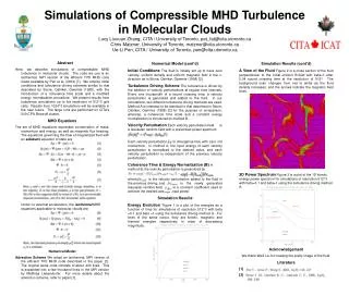
Simulations of Compressible MHD Turbulencein Molecular CloudsLucy Liuxuan Zhang, CITA / University of Toronto, pet_fat@cita.utoronto.caChris Matzner, University of Toronto, matzner@cita.utoronto.caUe-Li Pen, CITA / University of Toronto, pen@cita.utoronto.ca Abstract Here, we describe simulations of compressible MHD turbulence in molecular clouds. The code we use is an isothermal, MPI version of the efficient TVD MHD code made available by Pen et al. (2003) [1]. We employ initial conditions and turbulence driving schemes similar to that described by Stone, Ostriker, Gammie (1998), with the introduction of a coherence time scale and a modified energy normalization procedure. We present results from turbulence simulations up to the resolution of 512^3 grid cells. Results from 1024^3 simulations will be available in the near future. The large runs are performed on CITA's 540-CPU Beowulf cluster. MHD Equations The set of MHD equations expresses conservation of mass, momentum and energy, as well as magnetic flux freezing. The equations governing the flow of magnetized fluid with an adiabatic equation of state are Under no external acceleration, the isothermal MHD equations applicable to molecular clouds are Numerical Model Advection Scheme We adopt an isothermal, MPI version of the efficient TVD MHD code described in the paper [1]. The original serial code consists of about 400 lines. This is expanded into a few thousand lines in the MPI version by Matthias Liebendorfer. For more details about the advection scheme, refer to paper [1]. Numerical Model (cont’d) Initial Conditions The fluid is initially set up to have zero velocity, uniform density and uniform magnetic field in the x-direction as in Stone, Ostriker, Gammie (1998) [2]. Turbulence Driving Scheme The turbulence is driven by the addition of velocity perturbations at regular time intervals. Every one thousandth of a sound crossing time, a velocity perturbation is generated and added to the fluid. In our simulations, two different turbulence driving methods are used. Method A is intended to be identical to that described in Stone, Ostriker, Gammie (1998) [2] for the purpose of comparison; whereas, a coherence time scale and a constant energy normalization is introduced to method B. Velocity Perturbation Each velocity perturbation field is a Gaussian random field with a prescribed power spectrum Each velocity perturbation is divergence-free with zero net momentum. In method A, the input energy of each velocity perturbation is normalized to the desired value, and each velocity perturbation is independent of the previous velocity perturbation. Coherence Time & Energy Normalization (B) In method B, the velocity perturbation is prescribed by where is the velocity perturbation added to the fluid in the previous driving, and is the newly generated Gaussian random field. is a constant coefficient used to achieve the desired average input power. Simulation Results Energy Evolution Figure 1 is a plot of the energies as a function of time for simulations of resolution 512^3 with beta =0.1 and beta =1 using the turbulence driving method A. For lines of the same colour, they are kinetic, magnetic and thermal energies respectively in order of decreasing magnitude. Simulation Results (cont’d) A View of the Fluid Figure 2 is a cross section of the fluid perpendicular to the initial uniform B-field with beta=1 after 0.04 sound crossing time at the resolution of 5123. The background color changes from red to white as the fluid density increases, and the arrows indicate the magnetic field lines. 3D Power Spectrum Figure 3 is a plot of the 1D kinetic energy power spectrum for simulations of resolution 512^3 with beta=0.1 and beta=1 using the turbulence driving method A. Acknowledgement We thank Weili Liu for creating the pretty image of the fluid. Literature [1] [2]