Hypothesis Testing with t-Statistic in Statistics
520 likes | 543 Views
Learn how t-statistic is used in hypothesis testing when population standard deviation is unknown. Includes detailed steps and examples.

Hypothesis Testing with t-Statistic in Statistics
E N D
Presentation Transcript
Preview-1 • In the previous chapter, we presented the statistical procedure that permit researcher to use sample mean to test hypothesis about an unknown population • Remember that the expected value of the distribution of sample means is μ, the population mean σ σM = √n M - μ z = σM
THE PROBLEM WITH z-SCORE • A z-score requires that we know the value of the population standard deviation (or variance), which is needed to compute the standard error • In most situation, however, the standard deviation for the population is not known • In this case, we cannot compute the standard error and z-score for hypothesis test. We use t statistic for hypothesis testing when the population standard deviation is unknown
THE t STATISTIC:AN ALTERNATIVE TO z The goal of the hypothesis test is to determine whether or not the obtained result is significantly greater than would be expected by chance.
σ σM = √n s SM = √n Introducing t Statistic Now we will estimates the standard error by simply substituting the sample variance or standard deviation in place of the unknown population value Notice that the symbol for estimated standard error of M is SM instead of σM, indicating that the estimated value is computed from sample data rather than from the actual population parameter
z-score and t statistic σ s σM = SM = √n √n M - μ M - μ t = z = σM SM
The t Distribution • Every sample from a population can be used to compute a z-score or a statistic • If you select all possible samples of a particular size (n), then the entire set of resulting z-scores will form a z-scoredistribution • In the same way, the set of all possible t statistic will form a t distribution
The Shape of the t Distribution • The exact shape of a t distribution changes with degree of freedom • There is a different sampling distribution of t (a distribution of all possible sample t values) for each possible number of degrees of freedom • As df gets very large, then t distribution gets closer in shape to a normal z-score distribution
HYPOTHESIS TESTS WITH t STATISTIC • The goal is to use a sample from the treated population (a treated sample) as the determining whether or not the treatment has any effect Unknown population after treatment Known population before treatment TREATMENT μ = 30 μ = ?
HYPOTHESIS TESTS WITH t STATISTIC • As always, the null hypothesis states that the treatment has no effect; specifically H0 states that the population mean is unchanged • The sample data provides a specific value for the sample mean; the variance and estimated standard error are computed sample mean (from data) - population mean (hypothesized from H0) t = Estimated standard error (computed from the sample data)
LEARNING CHECK A psychologist has prepared an “Optimism Test” that is administered yearly to graduating college seniors. The test measures how each graduating class feels about it future. The higher the score, the more optimistic the class. Last year’s class had a mean score of μ = 19. A sample of n = 9 seniors from this years class was selected and tested. The scores for these seniors are as follow: 19 24 23 27 19 20 27 21 18 On the basis of this sample, can the psychologist conclude that this year’s class has a different level of optimism than last year’s class?
STEP-1: State the Hypothesis, and select an alpha level • H0 : μ = 19 (there is no change) • H1 : μ≠ 19 (this year’s mean is different) • Example we use α = .05 two tail
STEP-2: Locate the critical region • Remember that for hypothesis test with t statistic, we must consult the t distribution table to find the critical t value. With a sample of n = 9 students, the t statistic will have degrees of freedom equal to df = n – 1 = 9 – 1 = 8 • For a two tailed test with α = .05 and df = 8, the critical values are t = ± 2.306. The obtained t value must be more extreme than either of these critical values to reject H0
STEP-3: Obtain the sample data, and compute the test statistic • Find the sample mean • Find the sample variances • Find the estimated standard error SM • Find the t statistic s SM = √n M - μ t = SM
STEP-4: Make a decision about H0, and state conclusion • The obtained t statistic (t = 2.626) is in the critical region. Thus our sample data are unusual enough to reject the null hypothesis at the .05 level of significance. • We can conclude that there is a significant difference in level of optimism between this year’s and last year’s graduating classes t(8) = 2.626, p<.05, two tailed
The critical region in thet distribution for α= .05 and df= 8 Reject H0 Reject H0 Fail to reject H0 -2.306 2.306
DIRECTIONAL HYPOTHESES AND ONE-TAILED TEST • The non directional (two-tailed) test is more commonly used than the directional (one-tailed) alternative • On other hand, a directional test may be used in some research situations, such as exploratory investigation or pilot studies or when there is a priori justification (for example, a theory previous findings)
LEARNING CHECK A fund raiser for a charitable organization has set a goal of averaging at least $ 25 per donation. To see if the goal is being met, a random sample of recent donation is selected. The data for this sample are as follows: 20 50 30 25 15 20 40 50 10 20
The critical region in thet distribution for α = .05 and df = 9 Reject H0 Fail to reject H0 1.883
Preview-2 • In many research situations, however, its difficult or impossible for a researcher to satisfy completely the rigorous requirement of an experiment • In these situations, a researcher can often devise a research strategy (a method of collecting data) that is similar to an experiment but fails to satisfy at least one of the requirement of a true experiment
NonExperimental and Quasi Experimental • Although these studies resemble experiment, they always contain a confounding variable or other threat to internal validity that is an integral part of the design and simply cannot be removed • The existence of a confounding variable means that these studies cannot establish unambiguous cause-and-effect relationship and, therefore, are not true experiment
NonExperimental and Quasi Experimental • … is the degree to which the research strategy limits the confounding and control threats to internal validity • If a research design makes little or no attempt to minimize threats, it is classified as nonexperimental • A quasi experimental design makes some attempt to minimize threats to internal validity and approach the rigor of a true experiment
In an experiment… • … a researcher typically creates treatment condition by manipulating an IV, then measures participants to obtain a set of scores within each condition • If the score in one condition are significantly different from the other score in another condition, the researcher can conclude that the two treatment condition have different effects
NonExperimental and Quasi Experimental • Similarly, a nonexperimental study also produces group of scores to be compared for significant differences • One variable is used to create groups or conditions, then a second variable is measured to obtain a set of scores within each condition
NonExperimental and Quasi Experimental • In nonexperimental and quasi-experimental studies, the different groups or conditions are not created by manipulating an IV • The groups usually defined in terms of a preexisting participant variable (male/female) or in term of time (before/after)
Single sample techniques are used occasionally in real research, most research studies require the comparison of two (or more) sets of data • There are two general research strategies that can be used to obtain of the two sets of data to be compared: • The two sets of data come from the two completely separate samples (independent-measures or between-subjects design) • The two sets of data could both come from the same sample (repeated-measures or within subject design)
Taught by Method A Taught by Method B Do the achievement scores for students taught by method A differ from the scores for students taught by method B? In statistical terms, are the two population means the same or different? Unknown µ =? Unknown µ =? Sample A Sample B
THE HYPOTHESES FOR AN INDEPENDENT-MEASURES TEST • The goal of an independent-measures research study is to evaluate the mean difference between two population (or between two treatment conditions) H0: µ1 - µ2 = 0 (No difference between the population means) H1: µ1 - µ2 ≠ 0 (There is a mean difference)
THE FORMULA FOR AN INDEPENDENT-MEASURES HYPOTHESIS TEST • In this formula, the value of M1 – M2 is obtained from the sample data and the value for µ1 - µ2 comes from the null hypothesis • The null hypothesis sets the population mean different equal to zero, so the independent-measures t formula can be simplifier further - sample mean difference population mean difference M1 – M2 t = = S (M1 – M2) estimated standard error
THE STANDARD ERROR To develop the formula for S(M1 – M2)we will consider the following points: • Each of the two sample means represent its own population mean, but in each case there is some error s2 s12 s22 SM = SM1-M2 = + n √ √ n1 n2
POOLED VARIANCE • The standard error is limited to situation in which the two samples are exactly the same size (that is n1 – n2) • In situations in which the two sample size are different, the formula is biased and, therefore, inappropriate • The bias come from the fact that the formula treats the two sample variance
POOLED VARIANCE • for the independent-measure t statistic, there are two SS values and two df values SS s12 s22 SP2 = SM1-M2 = + n √ n1 n2
HYPOTHESIS TEST WITH THE INDEPENDENT-MEASURES t STATISTIC In a study of jury behavior, two samples of participants were provided details about a trial in which the defendant was obviously guilty. Although Group-2 received the same details as Group-1, the second group was also told that some evidence had been withheld from the jury by the judge. Later participants were asked to recommend a jail sentence. The length of term suggested by each participant is presented. Is there a significant difference between the two groups in their responses?
THE LENGTH OF TERM SUGGESTED BY EACH PARTICIPANT Group-1 scores: 4 4 3 2 5 1 1 4 Group-2 scores: 3 7 8 5 4 7 6 8 There are two separate samples in this study. Therefore the analysis will use the independent-measure t test
STEP-1: State the Hypothesis, and select an alpha level • H0 : μ1 - μ2 = 0 (for the population, knowing evidence has been withheld has no effect on the suggested sentence) • H1 : μ1 - μ2 ≠ 0 (for the population, knowledge of withheld evidence has an effect on the jury’s response) • We will set α = .05 two tail
STEP-2: Identify the critical region • For the independent-measure t statistic, degrees of freedom are determined by df = n1 + n2 – 2 = 8 + 8 – 2 = 14 • The t distribution table is consulted, for a two tailed test with α = .05 and df = 14, the critical values are t = ± 2.145. • The obtained t value must be more extreme than either of these critical values to reject H0
STEP-3: Compute the test statistic • Find the sample mean for each group M1 = 3 and M2 = 6 • Find the SS for each group SS1 = 16 and SS2 = 24 • Find the pooled variance, and SP2 = 2.86 • Find estimated standard error S(M1-M2) = 0.85
STEP-3: Compute the t statistic M1 – M2 -3 t = = = -3.55 S (M1 – M2) 0.85
STEP-4: Make a decision about H0, and state conclusion • The obtained t statistic (t = -3.53) is in the critical region on the left tail (critical t = ± 2.145). Therefore, the null hypothesis is rejected. • The participants that were informed about the withheld evidence gave significantly longer sentences, t(14) = -3.55, p<.05, two tails
The critical region in thet distribution for α= .05 and df= 14 Reject H0 Reject H0 Fail to reject H0 -2.145 2.145
LEARNING CHECK The following data are from two separate independent-measures experiments. Without doing any calculation, which experiment is more likely to demonstrate a significant difference between treatment A and B? Explain your answer.
LEARNING CHECK A psychologist studying human memory, would like to examine the process of forgetting. One group of participants is required to memorize a list of words in the evening just before going to bed. Their recall is tested 10 hours latter in the morning. Participants in the second group memorized the same list of words in he morning, and then their memories tested 10 hours later after being awake all day.
LEARNING CHECK The psychologist hypothesizes that there will be less forgetting during less forgetting during sleep than a busy day. The recall scores for two samples of college students are follows:
LEARNING CHECK • Sketch a frequency distribution for the ‘asleep’ group. On the same graph (in different color), sketch the distribution for the ‘awake’ group. Just by looking at these two distributions, would you predict a significant differences between two treatment conditions? • Use the independent-measures t statistic to determines whether there is a significant difference between the treatments. Conduct the test with α = .05
OVERVIEW • With a repeated-measures design, two sets of data are obtained from the same sample of individuals • The main advantage of a repeated-measures design is that it uses exactly the same individual in all treatment conditions.
The Hypotheses for a Related-Samples Test • As always, the null hypotheses states that for the general population there is no effect, no change, or no difference. H0: X2 - X1 = μD = 0 • The alternative hypotheses states that there is a treatment effect that causes the scores in one treatment condition to be systematically higher (or lower) than the scores in the other condition. In symbols H1: μD ≠ 0
The t Statistic for Related Samples • The t statistic for related samples is structurally similar to the other t statistics • One major distinction of the related samples t is that is based on difference scores rather than raw scores (X values)
The t Statistic for Related Samples - sample statistic population parameter or MD – μD t = = estimated standard error SMD S SMD = SS SS or SS √ df S2= S = = √ n-1 df df S2 SMD = √ n-1