第五章 特征值与特征向量 —— 幂法 /* Power Method */
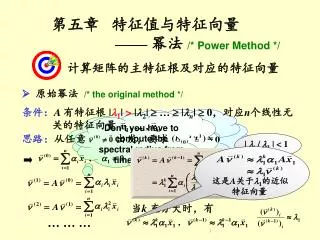
计算矩阵的主特征根及对应的特征向量. 条件: A 有特征根 | 1 | > | 2 | … | n | 0 , 对应 n 个线性无关的特征向量. 思路: 从任意 出发,要求. 这是 A 关于 1 的近似 特征向量. 第五章 特征值与特征向量 —— 幂法 /* Power Method */. 原始幂法 /* the original method */. Why in the earth do I want to know that?.

第五章 特征值与特征向量 —— 幂法 /* Power Method */
E N D
Presentation Transcript
计算矩阵的主特征根及对应的特征向量 条件:A 有特征根 |1| > |2| … |n| 0,对应n个线性无关的特征向量 思路:从任意 出发,要求 这是A关于1的近似 特征向量 第五章 特征值与特征向量 —— 幂法 /* Power Method */ 原始幂法 /* the original method */ Why in the earth do I want to know that? That is the eigenvalue with the largest magnitude. Don’t you have to compute the spectral radius from time to time? Wait a second, what does that dominant eigenvaluemean? | i / 1 | < 1 当k充分大时,有 … … …
Ch.5 Power Method – The Original Method 定理 设 ARnn为非亏损矩阵/* non-derogatory */,其主特征根 /* dominant eigenvalue */1为实根,且|1| > |2| … |n| 。则从任意非零向量 (满足 )出发, 迭代 收敛到主特征向量 , 收敛到1。 注: 结论对重根1 = 2 = … = r成立。 任取初始向量时,因为不知道 ,所以不能保证 1 0,故所求得之 不一定是 ,而是使得 的第一个 ,同时得到的特征根是m 。 每个不同的特征根只对应一个Jordan块 HW: p.98 #1 若有 1 = 2 ,则此法不收敛。
Ch.5 Power Method – Normalization 为避免大数出现,需将迭代向量规范化,即每一步先保证 ,再代入下一步迭代。一般用 。 记: 则有: 规范化 /* normalization */ Algorithm: Power Method To approximate the dominant eigenvalue and an associated eigenvector of the nn matrix A given a nonzero initial vector. Input: dimension n; matrix a[ ][ ]; initial vector V0[ ]; tolerance TOL; maximum number of iterations Nmax. Output: approximate eigenvalue and approximate eigenvector (normalized) or a message of failure.
Ch.5 Power Method – Normalization Algorithm: Power Method (continued) Step 1 Set k = 1; Step 2 Find index such that | V0[ index ] | = || V0 || ; Step 3 Set V0[ ] = V0[ ] / V0[ index ]; /* normalize V0 */ Step 4 While ( k Nmax) do steps 5-11 Step 5 V [ ] = A V0[ ]; /* compute Vk from Uk1 */ Step 6 = V[ index ]; Step 7Find index such that | V[ index ] | = || V || ; Step 8 If V[ index ] == 0 then Output ( “A has the eigenvalue 0”; V0[ ] ) ; STOP. /* the matrix is singular and user should try a new V0 */ Step 9err = || V0 V / V[ index ] || ; V0[ ] = V[ ] / V[ index ]; /* compute Uk */ Step 10 If (err < TOL) then Output( ; V0[ ] ) ; STOP. /* successful */ Step 11 Set k ++; Step 12 Output (Maximum number of iterations exceeded); STOP. /* unsuccessful */
Ch.5 Power Method – Deflation Technique 思路 令 B = A pI,则有 | IA | = | I(B+pI) | = | (p)IB | A p = B。而 ,所以求B的特征根收敛快。 希望 | 2 / 1 |越小越好。 n 2 1 As far as the laws of mathematics refer to reality, they are not certain, and as far as they are certain, they do not refer to reality. -- Albert Einstein (1879-1955) O 原点平移法/* deflation technique */ 不妨设 1 > 2 … n,且 | 2 |> | n |。 决定收敛的速度,特别 是 | 2 / 1 | p = ( 2+n ) / 2 How are we supposed to know where p is?
Ch.5 Power Method –Inverse Power Method 1 1 1 > … 若A 有| 1 | | 2 | … > |n |,则 A1 有 对应同样一组特征向量。 l l l - 1 n n 1 A1 的主特征根 A的绝对值最小的特征根 Q: How must we compute in every step? A: Solve a linear system with A factorized. 思路 反幂法/* Inverse Power Method */ 若知道某一特征根 i的大致位置 p,即对任意 j i有|i p | << |j p | ,并且如果 (A pI)1存在,则可以用反幂法求(A pI)1的主特征根 1/(i p) ,收敛将非常快。
Ch.5 Power Method –Inverse Power Method Lab 09. Approximating Eigenvalues Approximate an eigenvalue and an associated eigenvector of a given nn matrix A near a given value p and a nonzero vector . Input There are several sets of inputs. For each set: The 1st line contains an integer 100 n 0 which is the size of a matrix. n = 1 signals the end of file. The following n lines contain the matrix entries in the format shown: The next line contains a real number TOL, which is the tolerance for eigenvalues, and an integer N 0 which is the maximum number of iterations. The next line contains an integer nm > 0 which is the number of eigenvalues to be approximated. Each of the following m lines contains a real number p which is an initial approximation of the eigenvalue, followed by n real number entries of the nonzero vector . The numbers are separated by spaces and new lines. The inputs guarantee that the shifted matrix can be factorized by Doolittle method.
Ch.5 Power Method –Inverse Power Method • Output ( represents a space) • For each p, there must be a set of outputs in the following format: • The 1st line contains the approximation of an eigenvalue printed as in the C printf: fprintf(outfile, "%12.8f\n", lambda ); • The 2nd line contains the n entries of the associated eigenvector. Each entry is printed as in the C fprintf: fprintf(outfile, "%12.8f", x ); • If the method fails to give a solution after N iterations, print the message “Maximumnumberof iterationsexceeded.\n”. • If p is just the accurate eigenvalue, print the message • fprintf(outfile, “%12.8fisaneigenvalue.\n”, p ); • The outputs of two test cases must be seperated by a blank line. Sample Input 3 123 234 345 0.00000000011000 1 –0.6111 2 01 10 0.000000000110 1 1.011 –1 Sample Output –0.62347538 1.000000000.17206558–0.65586885 1.00000000isaneigenvalue.