4-25
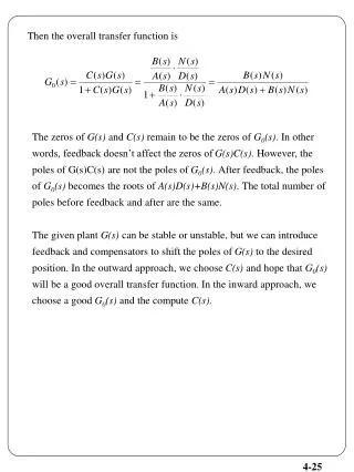
Then the overall transfer function is. The zeros of G(s) and C(s) remain to be the zeros of G 0 (s) . In other words, feedback doesn’t affect the zeros of G(s)C(s) . However, the poles of G(s)C(s) are not the poles of G 0 (s) . After feedback, the poles

4-25
E N D
Presentation Transcript
Then the overall transfer function is The zeros of G(s) and C(s) remain to be the zeros of G0(s).In other words, feedback doesn’t affect the zeros of G(s)C(s). However, the poles of G(s)C(s) are not the poles of G0(s).After feedback, the poles of G0(s) becomes the roots of A(s)D(s)+B(s)N(s). The total number of poles before feedback and after are the same. The given plant G(s) can be stable or unstable, but we can introduce feedback and compensators to shift the poles of G(s) to the desired position. In the outward approach, we choose C(s) and hope that G0(s) will be a good overall transfer function. In the inward approach, we choose a good G0(s) and the compute C(s). 4-25
Ch. 5 Frequency Domain Techniques 5.1 Introduction Here we’d like to introduce a design method based on the outward approach with the unity feedback configuration. The method uses G(jw) for all w0 where G(jw) can be obtained by direct measurement. The frequency response of a stable G(s) can be obtained by measurement. We apply u(t)=coswt and measure the steady state response. 5.2 Bode Plot Consider or Then we have the polar plot (a), the log magnitude-phase plot (b), and the Bode plot (c). It is clear that if any plot is available, then the other plot can be obtained. Here, we discuss the Bode plot only due to its mechanism for identifying a system and its usefulness in design. 5-1
Given a stable system with u(t)=ccoswo(t), then Let then The plots of |G(jw)|dB versus w and G(jw) versus w with w on a logarithmic scale are called the Bode plot of the system. Though the Bode plot can be easily obtained on a PC, it can be done by hand. Consider the transfer function H(s). Sketching the log-magnitude and phase frequency response curves as functions of logw can be simplified because these relationships can be approximated as a sequences of straight lines. - Construction of Bode Plots via Asymptotes |H(w)|dB = 20 log|H(w)| H(w) where the scale for w is logarithmic. Approximated by straight lines : asymptotes Consider 5-2
where Since logAB = logA + logB, Constant factors corner frequency (jwT+1) factors let then 5-3
Fig. 27. Magnitude (a) and phase (b) plots for the factor jwT+1 jw factors 20dB/decade w=1 0dB 5-4 Fig. 28. Magnitude (a) and phase (b) plots for the factor jw
Plotting Bode diagram (ex) Writing H(w) in the standard form yields Fig. 29. Magnitude (a) and phase (b) asymptotes 5-5
Fig. 30. Summed asymptotes and exact Bode diagrams Complex poles or zeros : Define corner frequency to be Then 5-6
40dB/decade Fig. 31. Magnitude (a) and phase (b) asymptote approximations for the quadratic term. However the exact Bode Diagram depends on the value of Fig. 32. Exact Bode diagram for a quadratic term. 5-7
0 -20 -40 w (ex) Consider 5-8
Fig. 33. Asymptotes and exact Bode plots for Example (a) magnitude (b) phase (1) Nonminimum phase transfer function Definition : A proper rational transfer function is called a minimum phase transfer function if all zeros lie inside the open left half s-plane. Otherwise, it is called a nonminimum phase transfer function. If zeros in the closed right half plane are called nonminimum phase zeros. Zeros in the open left half plane are called minimum phase zeros. (2) Identification Determination of the transfer function G(s) of a system from measured data is an identification problem. It is still possible to identify G(s) if G(s) has only one unstable pole at s=0. 5-9
(ex) Find the transfer function of the Bode plot shown below. First we approximate the gain plot by 3 straight lines. They intersect at w=1 and w=10. There is a straight line with slope -20dB/decade, therefore the transfer function has one pole at s=0. At w=1, the slope becomes -40dB/decade, thus there is a pole with corner frequency w=1. At w=10, the slope becomes -20dB/decade, there is a zero with corner frequency w=0. Thus the transfer function must be We know that the gain is 37dB at w=1. Thus Therefore, 5-10
Now we use the phase plot to determine the signs of each terms. For If K is negative the phase of is +900 and if K is positive, the phase is -900. From the phase plot, we conclude that K is positive and equals 99.6 If the sign of pole for (1s) is negative, the pole will introduce positive phase into G(s) and the phase of G(s) will increase as w passes through the corner frequency 1. This is not the case as shown in the phase plot. Thus we have 1+s. If the sign of zero for (10.1s) is positive, the zero will introduce positive phase into G(s) and the phase of G(s) will increase as w passes through the corner frequency at w=10. Obviously this is not the case. Thus we have 10.1s. Therefore, we have If the Bode Plot is obtained from measurement, then except for a possible pole at s=0, the system must be stable. Therefore, we can simply assign positive sign to the poles without checking the phase plot. If the transfer function is known to be of minimum phase, then we can assign positive sign to the zeros without checking the phase plot. In fact, if a transfer function is stable and of minimum phase, then there is unique relationship between the gain plot and phase plot, and we can determine the transfer function from the gain plot alone. 5-11
5.3 Frequency-Domain Specifications for Overall Systems Problem : Given a plant with transfer function G(s), design a feedback system with transfer function to meet a set of specifications. Specifications are generally stated in terms of position error, settling time, overshoot : time-domain specifications. If the design is to be carried out using frequency plots, we must translate the time domain specifications into the frequency domain. - Steady state performance Let be written as Typical amplitude and phase plots of control system are shown below. The steady-state error due to a step input is 5-12
The steady-state error due to a ramp input is We recognize that the steady state performance can be evaluated from - Transient performance The specifications consist of overshoot, settling time, and rise time. These specifications are related to and where The bandwidth is the frequency range in which the magnitude of is equal to or larger than . The frequency with the property is called the cutoff frequency. If then, Since the power is proportional to , the power of is also called the half-power point. Consider the following quadratic transfer function ----- Then, and 5-13
By simple manipulations, we show We know from time domain representation Overshoot = Now we plot two characteristic curves below. Fig 34. Peak resonance and overshoot. Then we have the relationship between overshoot and peak resonance. For example, if we require the overshoot less than 20%, then from the above figure, we see that must less than 1.25. Note that the peak resonance dictates the overshoot. The bandwidth of is related to the speed of response. The larger the bandwidth, the faster the response. Since the exact relationship is not known, we show a plausible argument of the statement for the quadratic transfer function. From the figure below, we note that the rise time inversely proportional to . 5-14
Fig 35 Responses of quadratic system with various damping ratios. The Bode plot of is shown below. The intersection of the -3dB line with the gain plot yields the cutoff frequency and the bandwidth. Since the bandwidth is proportional to , we conclude that the larger the bandwidth, the smaller the rise time or the faster the response. 5-15 Fig 36. Bode plot of quadratic term.
We often impose constraint on at high frequency. For example, we may require , for all Fig 37. Two frequency plots with same bandwidth. For the same bandwidth, if is closer to the cutoff frequency, then the cutoff rate of the gain plot will be larger. Note that the cutoff rate is the slope of the amplitude plot outside the bandwidth. The implification of this high frequency specification on the time response is not clear. However, it is related to noise rejection. 5.4 Frequency-Domain Specifications for Loop Transfer function : Unity-feedback Configuration. Problem : Given a plant with frequency-domain plot , design a system such that the overall transfer function will meet the specifications. The first approach is to compute for a chosen configuration. If doesn’t meet the specifications, we introduce a compensator and recompute . The second is to translate the specifications of into a set of for . If doesn’t meet the specifications, we introduce a compensator so that will meet the specifications. Because the first apporoach is much more complicated than the second one, it is rarely used in practice. 5-16
We shall use the unity-feedback configuration to take the second approach. + u y r C(s) G(s) _ Define Then - Steady state performance Consider We define We know that Assume that r(t)=1. Then, using the final value theorem, we have 5-17
Now assume that r(t)=t, then we show The relationship between the steady state specification and loop transfer functions via is shown below. - Transient performance The transient performance of is specified in terms of , bandwidth, and high frequency gain. Now, we translate these into a set of specifications for . However, we need to establish the relationship between . Consider . Then the vector drawn from (-1,0) to equal Their ratio 5-18
Let be a point of . Then Let Then With some algebraic manipulation, we show It is the equation of a circle with radius and centered at A family of such circles for various M is shown below. They are called the constant M-loci. If the constant M-loci is superposed on the polar plot of as shown, then can be read out directly. The circle with the largest M which polar plot of touches tangentially yields the peak resonance . 5-19 Fig 38. Constant M-loci
To see the relationship between the peak resonance and phase and gain margin, we show the following figure. Fig 39 Constant M-loci and phase and gain margins. From the intersection of M=1.2 with the real axis and the unit circle, we conclude that if gain margin of is smaller than 5.3dB or the phase of is smaller than , then peak resonance must be at least 1.2. Conversely we have Gain margin 10dB, Phase margin and Gain margin 12dB, Phase margin 5-20
Using the above figure, we can read the bandwidth of from the polar plot of If the cutoff frequency is the frequency at which the polar plot intersects with M circle of 0.7. As w increases, the polar plot first passes through the unit circle and then through the M-circle of 0.7, thus where is the gain crossover frequency of If an overall system is required to respond as fast as possible, then we may search for a compensator C(s) so that has a gain-crossover frequency as large as possible. The high frequency specifications on can be translated into that of . If G(s) is strictly proper and if C(s) is proper, then for large w.Thus we have Here the specification can be translate to The overall discussion is shown in the table below. Frequency Domain Time Domain Overall System Overall System Loop Transfer Function Position error Velocity error Steady-State Performance Transient Performance Overshoot Rise time Settling time Peak resonance Bandwidth High-frequency gain Gain and Phase margins Gain crossover frequency High-frequency gain 5-21