Download

1 / 61
610 likes | 911 Views
MATHEMATICAL PROPERTIES OF NETWORK OF PROTEIN INTERACTIONS . Abhishek Rathod CS 374 Algorithms in Biology Prof. Serafim Batzoglou . Broad plan . Part A Basics of Protein Interaction Networks and some background

E N D
MATHEMATICAL PROPERTIES OF NETWORK OF PROTEIN INTERACTIONS Abhishek Rathod CS 374 Algorithms in Biology Prof. Serafim Batzoglou
Broad plan • Part A Basics of Protein Interaction Networks and some background • 1.> JHU Lecture notes on “Computational Aspects of Molecular Structure- lecture notes” http://www.apl.jhu.edu/~przytyck/CAMS_lectures.html • 2.>And some figures and diagrams from random places… • Part B Network Biology • 1.>Network Biology: Understanding the cell’s functional organization • - Barabasi, Oltvai • 2.>The structure and function of complex networks -Newman • 3.>Knowledge Discovery in Proteomics: Graph theory Analysis of Protein Protein Interactions – Natasa Przulj • Part C Dynamically organized modularity in yeast proteome • 1.>Evidence for dynamically organized modularity in the yeast protein-protein interaction network – Han et.al. • Part D All with a pinch of salt… • 1.>Subnets of scale-free networks are not scale-free: Sampling properties of networks – Stumpf et.al. • 2.>Effect of sampling on topology predictions of protein-protein interaction networks – Han et.al. • Part E Conclusions and Future Directions
Biological Terminology • Protein complex • Domain • Molecular Pathway • Homology • Orthology • Paralogy
Graph Terminology Node Edge Directed/Undirected Degree Shortest Path/Geodesic distance Neighborhood Subgraph Complete Graph Clique Degree Distribution Hubs
Part A Examples of Biological Networks • Protein-Protein Interaction Networks • Metabolic Networks • Signaling Networks • Transcription Regulatory Networks
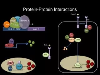
What is meant by a Protein-Protein Interaction (PPI) Network
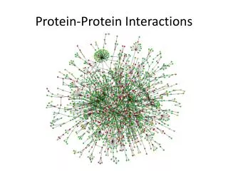
Example of a PPI Network • Yeast PPI network • Nodes – proteins • Edges – interactions The color of a node indicates the phenotypic effect of removing the corresponding protein (red = lethal, green = non-lethal, orange = slow growth, yellow = unknown).
Why is it useful to study PPI networks? • Proteins are workhorses of cell • Carry out catalytic reactions, transport, Form viral caspids • Transmit information from DNA to RNA, traverse membranes, • Form regulated channel, make possible synthesis of new proteins • Responsible for degradation of unnecessary proteins, vehicles of immune response • A prime way to predict protein function is through identification of binding partners • If the function of at least one of the components with which the protein interacts is known, that should let us assign its function(s) and the pathway(s) • Hence, through the intricate network of these interactions we can map cellular pathways, their interconnectivities and their dynamic regulation
Why is it useful to study structure of PPI networks? • Common properties of biological networks • Can help us relate network structure to biological function • Protein’s relative position in a network • Correlate conserved functional modules with protein complexes
How do we know that proteins interact? (PPI Identification methods) • Two types: • In vivo (inside a living body) • 1.>Yeast 2 hybrid assay A comprehensive two-hybrid analysis to explore yeast protein interactome – Ito,et.al • 2.>Mass spectrometry Functional organization of the yeast proteome by systematic analysis of protein complexes – Gavin et.al. • 3.>Correlated m-rna expression Functional Discovery via a compendium of expression profiles – Hughes et.al. • 4.>Genetic interactions MIPS: A database for genomes and protein sequences – Mewes et.al. • In silico (computational predictions) • Phylogenetic profiles • Rosetta stone • Gene neighbors • Co-evolution • Gene clusters A summary of all these methods can be found in Comparative assessment of large-scale data sets of protein-protein interactions – von Mering
PPI Public data sets • 1.>The Munich Information Center for Protein Sequences (MIPS) http://mips.gsf.de • 2.>Yeast Proteomics Database (YPD) http://www.incyte.com/sequence/proteome/databases/YPD.html • 3.>Human Reference Protein Database (HRPD) http://www.hrpd.org • 4.>The Biomolecular Interaction Network Database http://www.binddb.org/ • 5.>The General Repository for Interaction Datasets (GRID) http://biodata.mshri.on.ca/grid/ • 6.>The Molecular INTeraction database (MINT) mint.bio.uniroma2.it/mint/ • 7.>Online Predicted Human Interaction Database (OPHID) http://ophid.utoronto.ca
Problem of false positives and false negatives 1 • Coverage of The yeast, C.Elegans and Drosophila interactome maps are mere 3-9% of the incomplete interactome. • This low coverage explains limited overlap observed between different data sets • False negative can arise from • Biased or limited coverage • False positives can arise from • Limitations in experimental procedure used • Absence of cellular milieu
Aims of Network Theory PART B 1.>Find statistical properties that characterize the structure and behavior of networked systems 2.> Create models of networks that can help us to understand the meaning of these properties 3.> Predict what the behavior of networked systems will be One of the principal thrusts of recent work in this area is inspired by groundbreaking paper by Watts and Strogatz1. • 1.Collective dynamics of small world networks – Watts, Strogatz
Types of networks 1 A. Social Network Examples: the patterns of friendships between individuals, business relationships between companies and intermarriages between families B. Information Network Examples: Citation Network, World Wide Web
Types of Networks 2 C Technological Networks Examples Electric power grid, network of airline routes, roads and railways, river networks D Biological Networks Protein Interaction Networks, metabolic pathways, gene regulatory networks, signaling pathways, food web, neural networks
Properties of networks • Small world effect • Transitivity/ Clustering • Scale Free Effect • Maximum degree • Network Resilience and robustness • Mixing patterns and assortativity • Degree correlations • Community structure • Evolutionary origin • Betweenness centrality of vertices
Small world effect • most pairs of vertices in the network seem to be connected by a short path • l is mean geodesic distance • dij is the geodesic distance between vertex i and vertex j • Effect on the dynamics of processes taking place on network • A more precise meaning to small world effect
Transitivity/Clustering • A network shows clustering if the probability of pair of nodes being adjacent is higher when the two nodes have a common neighbor. • Clustering coefficient C is defined as the average probability that two neighbors of a given node are adjacent. • The clustering coefficient C of the whole network is the average of Cvs for all nodes v in the network. • Ev is the number of edges between neighbors of v. • A node v has dv neighbors. • Complex Real world networks exhibit a large degree of clustering i.e. clustering coefficient is much higher than random graphs. • An important measure of network’s structure is the function Ck which is the average clustering coefficient of all nodes with k links. Graph with a big C
Network resilience and robustness- ITopological Robustness • Most of the networks we have been considering rely for their function on their connectivity. • Effect of removing vertices on shortest path length • For the graph of internet • The Internet is highly resilient against random failure of vertices but highly vulnerable to deliberate attack on its highest degree vertices.
Network resilience and robustness- IIFunctional and dynamic robustness • Effect of a perturbation cannot depend on the node’s degree only! • Experimentally identified protein complexes tend to be composed of uniformly essential or non-essential molecules • Effect of deviations in the rate constants or ligand concentrations on the chemotaxis receptor module of E. coli
Mixing patterns and Assortativity • In a food web, links between plants, herbivores and carnivores. • Links between users, ISP and backbones • In social networks this kind of selective linking is called assortative mixing or homophily • Disassortative nature of cellular networks:In protein interaction networks, highly connected nodes (hubs) avoid linking directly to each other and instead connect to proteins with only a few interactions
Community structure • “Community structure,” is a groups of vertices that have a high density of edges within them, with a lower density of edges between groups. • Example: Friendship network of children in a school • Other Examples • Citation networks:particular areas of research interest • World Wide Web:subject matter of pages • Communities in metabolic networks: Functional Units • Hierarchical clustering More properties?
Network Models • Random Network • Scale free Network • Hierarchical Network
Random Network I • The Erdös–Rényi (ER) model of a random network starts with N nodes and connects each pair of nodes with probability p, which creates a graph with approximately pN(N–1)/2 randomly placed links • The node degrees follow a Poisson distribution
Random Network II • Mean shortest path l ~ log N, which indicates that it is characterized by the small-world property. • Random graphs have served as idealized models of certain gene networks, ecosystems and the spread of infectious diseases and computer viruses.
Scale Free Networks I • P(k) ~ k –γ, where γ is the degree exponent. The network’s properties are determined by hubs The network is often generated by a growth process called Barabási–Albert model
Scale Free Networks II • Scale-free networks with degree exponents 2<γ<3, a range that is observed in most biological and non-biological networks like the Internet backbone, the World Wide Web, metabolic reaction network and telephone call graphs. • The mean shortest path length is proportional to log(n)/log(log(n))
Scale Free Networks III Scale Free Model as applied to Biological Network Example of a predicted pathway which has scale free topology • The analysis of metabolic networks of 43 organisms from the WIT database showed to have scale-free topology with P(k) ~k-2.2 for both in and out degrees. • The diameter of metabolic networks was the same • A few hubs dominated these networks and upon sequential removal of the most connected nodes the diameter rose sharply • Only around 4% of the nodes were present in all species and these were the ones that were most highly connected in any individual organism. • Randomly removing nodes from these networks, the average shortest path lengths did not change, indicating insensitivity to random errors in networks.
Hierarchical Networks I • To account for the coexistence of modularity, local clustering and scale-free topology in many real systems it has to be assumed that clusters combine in an iterative manner, generating a hierarchical network • The hierarchical network model seamlessly integrates a scale-free • topology with an inherent modular structure by generating a network that has a power-law degree distribution with degree exponent γ = 1 + ln4/ln3 = 2.26
Hierarchical Networks II • It has a large system-size independent average clustering coefficient <C> ~ 0.6. The most important signature of hierarchical modularity is the scaling of the clustering coefficient, which follows C(k) ~ k –1 a straight line of slope –1 on a log–log plot • A hierarchical architecture implies that sparsely connected nodes are part of highly clustered areas, with communication between the different highly clustered neighborhoods being maintained by a few hubs • Some examples of hierarchical scale free networks.
Hierarchical Networks III Hierarchical Model as applied to Biological Network • It was established that the model closely overlaps with E.Coli’s known metabolic network. • It is the MOST successful of all the network models in application to biological networks! Hierarchical networks were successful in modeling not only E.Coli’s metabolic network but networks of all 43 organisms earlier modeled by scale free networks.
Motifs, Modules and Hierarchical networks • Cellular functions are likely to be carried out in a highly modular manner. • High clustering => High modularity • Network motifs can be defined as patterns of interconnections that recur in many different parts of a network at frequencies much higher than those found in random networks. • These motifs are likely to be functional modules in which the cell operates • Each real network is characterized by its own set of distinct motifs • Motifs show higher degree of evolutionary conservation across diverse species. • Empirical observations indicate that motif aggregate to form large motif clusters which overlap and hence are no longer separable. • Here are three motifs that appear in E.Coli • Each motif in the above diagram has a specific function in determining gene expression.
Identification of Motifs: • Search for subgraphs combinatorially infeasible • Alternative 1- Identify group of highly connected nodes and correlate this entity with its potential functional role. • Alternative 2 – Look around a node with a low degree. • Alternative 3 – Clustering methods – homogeneity and separation • Problems with clustering methods • Different methods predict boundaries between modules that are not sharply separated • Changing an internal parameter within the method may result in larger or smaller module.
Function-Structure relationship in PPI networks: (Assuming functional classification in MIPS database) • Distinct functional classes of proteins have differing network properties. • Proteins involved in translation appear to have highest average degree while transport and sensing proteins have lowest average degree. • Metabolic networks across 43 organisms tested have an average degree < 4 • Amongst all functional groups, cellular organization proteins have largest presence in hub nodes whose removal disconnects the PPI network.
Part C Evidence for dynamically organized modularity in the yeast PPI network • Introduction • The aim of the paper is to investigate how hubs contribute to dynamically organized modularity in yeast networks • ‘Date hubs’ and ‘Party hubs’ They formulate a model in which date hubs organize the modules and party hubs function inside these modules
Obtaining Data • To minimize false positives they generated a high quality yeast interaction data set by intersecting data generated by several different interaction detection methods.
How are party hubs distinguished from date hubs? I • Pearson correlation coefficient (PCC) is calculated between hub and each of its respective partner. • Bimodal distribution. • The average PCCs of nonhubs show a normal distribution centered on 0.1 • In randomized interactome networks of the same topology the average PCCs of hubs show a normal distribution centered on 0.1 • Party hubs are those with an average PCC higher than the threshold in at least one of the five conditions. All other hubs are defined as date hubs. • Using this criteria they found 91 date hubs and 108 party hubs • The six experiments show dynamics of interactome networks expression timing.
How are party hubs distinguished from date hubs? II • Red curve – hubs • Cyan curve – nonhubs • Black curve - randomized • Arrow indicates -> threshold • The dynamics of interactome networks was also confirmed with spatial distribution i.e. subcellular localization. • Partners of date hubs are significantly more diverse in spatial distribution than partners of party hubs
Effect of removal of nodes on average geodesic Green – nonhub nodes Brown – hubs Red – date hubs Blue – party hubs The ‘breakdown point’ is the threshold after which the main component of the network starts disintegrating.
Network disintegration Original Network On removal of date hubs On removal of party hubs
Modular subnetsand Essentialilty • Use of annotations from MIPS database. • It was observed that subnetworks represent not only stable molecular machines or complexes but also more loosely connected regulatory pathways • Protein pairs inside subnetworks corresponding to protein complexes tend to show high PCC values • Less densely connected regulatory pathways tend to show lower PCC values • Essentiality • In single gene knockout experiments similar proportions of party and date hubs score as essential
Dynamically organized modularity! The results support a model of organized modularity for the yeast proteome where date hubs represent global or ‘higher level’ connectors between modules and party hubs function inside modules at a ‘lower level’ of the organization. Red circles – Date hubs Blue squares - Modules An example
Part D Subnets of scale free networks are not scale free: Sampling properties of networks • Only if the degree distributions of the network and randomly sampled subnets belong to the same family of probability distributions is it possible to extrapolate from subnet data to properties of global network. • The aim of this paper is to show that this condition is satisfied for random graphs and exponential random graphs but not for scale free degree distributions. • Method of sampling • Each node in N is included in the subnet S with probability p and left out of the subnet with probability (1 - p) • For finite networks, the expected size of the subnet is thus E[M] = Np with variance Var[M] =Np(1 - p). • The deviation from scale free behavior is more pronounced as power law exponent γ increases and as p decreases
Effect of sampling on topology predictions of PPI networks • Introduction • To extrapolate the topology of complete interactomes from such incomplete maps requires the assumption that limited sampling does not affect the overall topological analyses • It can be shown via in silico simulations that limited sampling alone can give rise to apparent scale free topologies irrespective of original network topology and thus complete network topologies cannot be extrapolated directly from the sub-network data. • The four distributions used are random networks (ER), Exponential networks (EN), Power Law (PL) and Truncated Normal (TN). • Sampling methodology • Given estimations of average <k> in the full yeast interactomes a model for complete interactomes with <k> of 5, 10 and 20 is chosen. • Network matching a predefined degree distribution formula for ER, PL, TN or EX distribution is generated by an edge allocation algorithm. • Sampling as it occurs in Y2H is done by simulating bait coverage and edge coverage. For each theoretical topology model bait and edge coverage ranges were scanned from 0 to 100%. • The linear regression R-square function is used to assess linearity from log(n(k)) and log(k). R-square ranges from 0 to 1 with 1 representing perfect linearity.
Results of sampling • Limited sampling alone can lead to misleading degree distribution. • Many technical false positives are auto activators or sticky proteins represented by nodes of artificially high degree, which might tilt apparent topology even more toward scale free than observed by sampling alone. • The scale free Internet and World Wide Web are necessarily sampled because of their vast size. In contrast with PPI networks, these networks may still be scale free because although node coverage is low, edge coverage by sampling methods used is close to 100%
Part E • Conclusions • Scale free networks are resistant to random failure but vulnerable to targeted attack, specifically against hubs. This property has been held to account for the robustness of biological networks to perturbations like mutation and environmental stress. A positive correlation between essentiality and connectivity has been demonstrated linking topological centrality to functional essentiality. • Whether you study the cell in a top-down manner or bottom-up manner the structural and topological properties of cellular networks must be considered • Given the current limited coverage levels, the observed scale-free topology of existing interactome maps cannot be confidently extrapolated to complete interactomes. • There is dire need to increase coverage through further experimentation, as well as through development of improved PPI mapping technology • We saw a model of organized modularity for the yeast proteome, with modules connected through regulators, mediators or adaptors, the date hubs • Party hubs represent integral elements within distinct modules and operate at lower level in the organization of the proteome.
Future Directions • New theoretical methods to characterize network topology • Improve understanding of dynamics of motif clusters and its biological function • Improve data collections abilities so that we have a higher resolution in space and time • Taking cell’s intercellular milieu, 3-d shape, anatomical architecture, compartmentalization and state of cytoskeleton into consideration while determining protein interactions. • A full description of protein interaction network requires that model would encompass interaction confidence level, source and multiplicity of an interaction, directional pathway information, temporal information about presence or absence of a PPI, information on strength of interactions etc. • To find an efficient and robust graph clustering algorithm that would reliably identify protein complexes • Modeling signaling pathways and finding efficient algorithms for their identification in PPI networks • The existence of “core proteome” has been hypothesized. It has been proposed that approximately 40% of yeast proteins are conserved through eukaryotic evolution. Verification of this claim is a challenge for network biology. • It is possible that discriminating between date and party hubs might help to define new therapeutic drug targets. • Network biology if used in a well-developed framework can be used to identify modules that are pathologically altered in a given disease. A framework for pharmaceutical modification of the diseased modules is needed.