Double Integrals and Volumes in Multiple Integrals
Explore the concept of double integrals and finding volumes of solids using Riemann sums. Learn how to calculate volumes above rectangles and below surface graphs in this detailed chapter.


Double Integrals and Volumes in Multiple Integrals
E N D
Presentation Transcript
2 MULTIPLE INTEGRALS
MULTIPLE INTEGRALS • In this chapter, we extend the idea of a definite integral to double and triple integrals of functions of two or three variables.
MULTIPLE INTEGRALS 2.1 Double Integrals over Rectangles In this section, we will learn about: Double integrals and using them to find volumes.
DOUBLE INTEGRALS OVER RECTANGLES • Just as our attempt to solve the area problem led to the definition of a definite integral, we now seek to find the volume of a solid. • In the process, we arrive at the definition of a double integral.
DEFINITE INTEGRAL—REVIEW • First, let’s recall the basic facts concerning definite integrals of functions of a single variable.
DEFINITE INTEGRAL—REVIEW • If f(x) is defined for a ≤x ≤b, we start by dividing the interval [a, b] into n subintervals [xi–1, xi] of equal width ∆x = (b –a)/n. • We choose sample points xi* in these subintervals.
DEFINITE INTEGRAL—REVIEW Equation 1 • Then, we form the Riemann sum
DEFINITE INTEGRAL—REVIEW Equation 2 • Then, we take the limit of such sums as n → ∞ to obtain the definite integral of ffrom a to b:
DEFINITE INTEGRAL—REVIEW • In the special case where f(x) ≥ 0, the Riemann sum can be interpreted as the sum of the areas of the approximating rectangles.
DEFINITE INTEGRAL—REVIEW • Then, represents the area under the curve y = f(x) from a to b.
VOLUMES • In a similar manner, we consider a function f of two variables defined on a closed rectangle • R = [a, b] x [c, d] • = {(x, y) € R2 | a ≤ x ≤ b, c ≤ y ≤ d • and we first suppose that f(x, y) ≥ 0. • The graph of f is a surface with equation z =f(x, y).
VOLUMES • Let S be the solid that lies above R and under the graph of f, that is, • S = {(x, y, z) R3 | 0 ≤ z ≤ f(x, y), (x, y) R} • Our goal is to find the volume of S.
VOLUMES • The first step is to divide the rectangle R into subrectangles. • We divide the interval [a, b] into m subintervals [xi–1, xi] of equal width ∆x = (b –a)/m. • Then, wedivide [c, d] into n subintervals [yj–1, yj]of equal width ∆y = (d –c)/n.
VOLUMES • Next, we draw lines parallel to the coordinate axes through the endpoints of these subintervals.
VOLUMES • Thus, we form the subrectangles Rij = [xi–1, xi]x [yj–1, yj] = {(x, y) | xi–1 ≤ x ≤ xi, yj–1 ≤ y ≤ yj} each with area ∆A =∆x ∆y
VOLUMES • Let’s choose a sample point (xij*, yij*) in each Rij.
VOLUMES • Then, we can approximate the part of S that lies above each Rij by a thin rectangular box (or “column”) with: • Base Rij • Height f (xij*, yij*)
VOLUMES • Compare the figure with the earlier one.
VOLUMES • The volume of this box is the height of the box times the area of the base rectangle: f(xij*, yij*) ∆A
VOLUMES • We follow this procedure for all the rectangles and add the volumes of the corresponding boxes.
VOLUMES Equation 3 • Thus, we get an approximation to the total volume of S:
VOLUMES Equation 4 • Our intuition tells us that the approximation given in Equation 3 becomes better as m and n become larger. • So, we would expect that:
VOLUMES • We use the expression in Equation 4 to define the volume of the solid S that lies under the graph of f and above the rectangle R.
DOUBLE INTEGRAL Definition 5 • The double integral of f over the rectangle Ris: • if this limit exists.
DOUBLE INTEGRAL • The sample point (xij*, yij*) can be chosen to be any point in the subrectangle Rij*.
DOUBLE INTEGRAL • If f(x, y) ≥ 0, then the volume V of the solid that lies above the rectangle R and below the surface z = f(x, y) is:
DOUBLE REIMANN SUM • The sum in Definition 5 • is called a double Riemann sum.
DOUBLE INTEGRALS Example 1 • Estimate the volume of the solid that lies above the square R = [0, 2] x [0, 2] and below the elliptic paraboloid z = 16 – x2 – 2y2. • Divide R into four equal squares and choose the sample point to be the upper right corner of each square Rij. • Sketch the solid and the approximating rectangular boxes.
DOUBLE INTEGRALS Example 1 • The squares are shown here. • The paraboloid is the graph of f(x, y) = 16 – x2 – 2y2 • The area of eachsquare is 1.
DOUBLE INTEGRALS Example 1 • Approximating the volume by the Riemann sum with m =n = 2, we have:
DOUBLE INTEGRALS Example 1 • That is the volume of the approximating rectangular boxes shown here.
DOUBLE INTEGRALS • We get better approximations to the volume in Example 1 if we increase the number of squares.
DOUBLE INTEGRALS • The figure shows how, when we use 16, 64, and 256 squares, • The columns start to look more like the actual solid. • The corresponding approximations get more accurate.
DOUBLE INTEGRALS • In Section 2.3, we will be able to show that the exact volume is 48.