MULTIPLE INTEGRALS
15. MULTIPLE INTEGRALS. MULTIPLE INTEGRALS. 15.3 Double Integrals over General Regions. In this section, we will learn: How to use double integrals to find the areas of regions of different shapes. SINGLE INTEGRALS.


MULTIPLE INTEGRALS
E N D
Presentation Transcript
15 MULTIPLE INTEGRALS
MULTIPLE INTEGRALS 15.3 Double Integrals over General Regions • In this section, we will learn: • How to use double integrals to find • the areas of regions of different shapes.
SINGLE INTEGRALS • For single integrals, the region over which we integrate is always an interval.
DOUBLE INTEGRALS • For double integrals, we want to be able to integrate a function f not just over rectangles but also over regions D of more general shape. • One such shape is illustrated.
DOUBLE INTEGRALS • We suppose that D is a bounded region. • This means that D can be enclosed in a rectangular region R as shown.
DOUBLE INTEGRALS Equation 1 • Then, we define a new function F with domain R by:
DOUBLE INTEGRAL Definition 2 • If F is integrable over R, then we define the double integral of f over D by: • where F is given by Equation 1.
DOUBLE INTEGRALS • Definition 2 makes sense because R is a rectangle and so has been previously defined in Section 15.1
DOUBLE INTEGRALS • The procedure that we have used is reasonable because the values of F(x, y) are 0 when (x, y) lies outside D—and so they contribute nothing to the integral. • This means that it doesn’t matter what rectangle R we use as long as it contains D.
DOUBLE INTEGRALS • In the case where f(x, y) ≥ 0, we can still interpret • as the volume of the solid that lies above D and under the surface z = f(x, y) (graph of f).
DOUBLE INTEGRALS • You can see that this is reasonable by: • Comparing the graphs of f and F here. • Remembering is the volume under the graph of F.
DOUBLE INTEGRALS • This figure also shows that F is likely to have discontinuities at the boundary points of D.
DOUBLE INTEGRALS • Nonetheless, if f is continuous on D and the boundary curve of D is “well behaved” (in a sense outside the scope of this book), then it can be shown that exists and so exists. • In particular, this is the case for the followingtypes of regions.
DOUBLE INTEGRALS • In particular, this is the case for the following types of regions.
TYPE I REGION • A plane region D is said to be of type Iif it lies between the graphs of two continuous functions of x, that is, • D = {(x, y) | a≤ x ≤ b, g1(x) ≤ y ≤ g2(x)} • where g1 and g2 are continuous on [a, b].
TYPE I REGIONS • Some examples of type I regions are shown.
TYPE I REGIONS • To evaluate when D is a region of type I, we choose a rectangle R = [a, b] x [c, d] that contains D.
TYPE I REGIONS • Then, we let F be the function given by Equation 1. • That is, F agrees with f on D and F is 0 outside D.
TYPE I REGIONS • Then, by Fubini’s Theorem,
TYPE I REGIONS • Observe that F(x, y) = 0 if y < g1(x) or y > g2(x) because (x, y) then lies outside D.
TYPE I REGIONS • Therefore, • because F(x, y) = f(x, y) when g1(x) ≤ y ≤ g2(x).
TYPE I REGIONS • Thus, we have the following formula that enables us to evaluate the double integral as an iterated integral.
TYPE I REGIONS Equation 3 • If f is continuous on a type I region D such that • D = {(x, y) | a≤ x ≤ b, g1(x) ≤ y ≤ g2(x)} • then
TYPE I REGIONS • The integral on the right side of Equation 3 is an iterated integral that is similar to the ones we considered in Section 15.3 • The exception is that, in the inner integral, we regard x as being constant not only in f(x, y) but also in the limits of integration, g1(x) and g2(x).
TYPE II REGIONS Equation 4 • We also consider plane regions of type II, which can be expressed as: • D = {(x, y) | c≤ y ≤ d, h1(y) ≤ x ≤ h2(y)} • where h1 and h2 are continuous.
TYPE II REGIONS • Two such regions are illustrated.
TYPE II REGIONS Equation 5 • Using the same methods that were used in establishing Equation 3, we can show that: • where D is a type II region given by Equation 4.
TYPE II REGIONS Example 1 • Evaluate where D is the region bounded by the parabolas y = 2x2 and y = 1 + x2.
TYPE II REGIONS Example 1 • The parabolas intersect when 2x2 = 1 + x2, that is, x2 = 1. • Thus, x = ±1.
TYPE II REGIONS Example 1 • We note that the region D is a type I region but not a type II region. • So, we can write: D = {(x, y) | –1 ≤ x ≤ 1, 2x2 ≤ y ≤ 1 + x2}
TYPE II REGIONS Example 1 • The lower boundary is y = 2x2 and the upper boundary is y = 1 + x2. • So,Equation 3 gives the following result.
TYPE II REGIONS Example 1
NOTE • When we set up a double integral as in Example 1, it is essential to draw a diagram. • Often, it is helpful to draw a vertical arrow as shown.
NOTE • Then, the limits of integration for the inner integral can be read from the diagram: • The arrow starts at the lower boundary y = g1(x), which gives the lower limit in the integral. • The arrow ends at the upper boundary y = g2(x), which gives the upper limit of integration.
NOTE • For a type II region, the arrow is drawn horizontally from the left boundary to the right boundary.
TYPE I REGIONS Example 2 • Find the volume of the solid that lies under the paraboloid z = x2 + y2 and above the region D in the xy–plane bounded by the line y = 2x and the parabola y = x2.
TYPE I REGIONS E. g. 2—Solution 1 • From the figure, we see that D is a type I region and D = {(x, y) | 0 ≤ x ≤ 2, x2 ≤ y ≤ 2x} • So, the volume under z = x2 + y2 and above Dis calculated as follows.
TYPE I REGIONS E. g. 2—Solution 1
TYPE I REGIONS E. g. 2—Solution 1
TYPE II REGIONS E. g. 2—Solution 2 • From this figure, we see that D can also be written as a type II region: D = {(x, y) | 0 ≤ y ≤ 4, ½y ≤ x ≤ • So, another expression for V is as follows.
TYPE II REGIONS E. g. 2—Solution 2
DOUBLE INTEGRALS • The figure shows the solid whose volume is calculated in Example 2. • It lies: • Above the xy-plane. • Below the paraboloid z = x2 + y2. • Between the plane y = 2x and the parabolic cylinder y = x2.
DOUBLE INTEGRALS Example 3 • Evaluate where D is the region bounded by the line y = x – 1 and the parabola y2 = 2x + 6
TYPE I & II REGIONS Example 3 • The region D is shown. • Again, D is both type I and type II.
TYPE I & II REGIONS Example 3 • However, the description of D as a type I region is more complicated because the lower boundary consists of two parts.
TYPE I & II REGIONS Example 3 • Hence, we prefer to express D as a type II region: • D = {(x, y) | –2 ≤ y ≤ 4, 1/2y2 – 3 ≤ x ≤ y + 1} • Thus, Equation 5 gives the following result.
TYPE I & II REGIONS Example 3
TYPE I & II REGIONS Example 3 • If we had expressed D as a type I region, we would have obtained: • However, this would have involved more work than the other method.
DOUBLE INTEGRALS Example 4 • Find the volume of the tetrahedron bounded by the planes • x + 2y + z = 2 • x = 2y • x = 0 • z = 0
DOUBLE INTEGRALS Example 4 • In a question such as this, it’s wise to draw two diagrams: • One of the three-dimensional solid • One of the plane region D over which it lies