Adversarial Search Game Playing
430 likes | 647 Views
Adversarial Search Game Playing. Chapter 6. Outline. Games Perfect Play Minimax decisions α-β pruning Resource Limits and Approximate Evaluation Games of chance. Games.

Adversarial Search Game Playing
E N D
Presentation Transcript
Adversarial Search Game Playing Chapter 6
Outline • Games • Perfect Play • Minimax decisions • α-β pruning • Resource Limits and Approximate Evaluation • Games of chance
Games • Multi agent environments : any given agent will need to consider the actions of other agents and how they affect its own welfare. • The unpredictability of these other agents can introduce many possible contingencies • There could be competitive or cooperative environments • Competitive environments, in which the agent’s goals are in conflict require adversarial search – these problems are called as games
What kind of games? • Abstraction: To describe a game we must capture every relevant aspect of the game. Such as: • Chess • Tic-tac-toe • … • Accessible environments: Such games are characterized by perfect information • Search: game-playing then consists of a search through possible game positions • Unpredictable opponent: introduces uncertainty thus game-playing must deal with contingency problems Slide adapted from Macskassy
Games • In game theory (economics), any multi-agent environment (either cooperative or competitive) is a game provided that the impact of each agent on the other is significant* • AI games are a specialized kind - deterministic, turn taking, two-player, zero sum games of perfect information • a zero-sum game is a mathematical representation of a situation in which a participant's gain (or loss) of utility is exactly balanced by the losses (or gains) of the utility of other participant(s) • In our terminology – deterministic, fully observable environments with two agents whose actions alternate and the utility values at the end of the game are always equal and opposite (+1 and –1) • If a player wins a game of chess (+1), the other player necessarily loses (-1) • * Environments with very many agents are best viewed as economies rather than games
Deterministic Games • Many possible formalizations, one is: • States: S (start at s0) • Players: P={1...N} (usually take turns) • Actions: A (may depend on player / state) • Transition Function: SxA →S • Terminal Test: S → {t,f} • Terminal Utilities: SxP → R • Solution for a player is a policy: S → A
Games vs. search problems • “Unpredictable" opponent solution is a strategy specifying a move for every possible opponent reply • Time limits unlikely to find goal, must approximate • Plan of attack: • Computer considers possible lines of play (Babbage, 1846) • Algorithm for perfect play (Zermelo, 1912; Von Neumann, 1944) • Finite horizon, approximate evaluation (Zuse, 1945; Wiener, 1948; Shannon, 1950) • First chess program (Turing, 1951) • Machine learning to improve evaluation accuracy (Samuel, 1952-57) • Pruning to allow deeper search (McCarthy, 1956)
Deterministic Single-Player? • Deterministic, single player, perfect information: • Know the rules • Know what actions do • Know when you win • E.g. Freecell, 8-Puzzle, Rubik’s cube • … it’s just search! • Slight reinterpretation: • Each node stores a value: the best outcome it can reach • This is the maximal outcome of its children (the max value) • Note that we don’t have path sums as before (utilities at end) • After search, can pick move that leads to best node Slide adapted from Macskassy
Deterministic Two-Player • E.g. tic-tac-toe, chess, checkers • Zero-sum games • One player maximizes result • The other minimizes result • Minimax search • A state-space search tree • Players alternate • Each layer, or ply, consists of a round of moves • Choose move to position with highest minimax value = best achievable utility against best play Slide adapted from Macskassy
Searching for the next move • Complexity: many games have a huge search space • Chess: b = 35, m=100 nodes = 35 100 • if each node takes about 1 ns to explore then each move will take about 1050millennia to calculate. • Resource (e.g., time, memory) limit: optimal solution not feasible/possible, thus must approximate • 1. Pruning: makes the search more efficient by discarding portions of the search tree that cannot improve quality result. • 2. Evaluation functions: heuristics to evaluate utility of a state without exhaustive search. Slide adapted from Macskassy
Two-player Games • A game formulated as a search problem: Slide adapted from Macskassy
The minimax algorithm • Perfect play for deterministic environments with perfect information • Basic idea: choose move with highest minimax value = best achievable payoff against best play • Algorithm: 1. Generate game tree completely 2. Determine utility of each terminal state 3. Propagate the utility values upward in the three by applying MIN and MAX operators on the nodes in the current level 4. At the root node use minimax decision to select the move with the max (of the min) utility value • Steps 2 and 3 in the algorithm assume that the opponent will play perfectly.
Minimax value • Given a game tree, the optimal strategy can be determined by examining the minimax value of each node (MINIMAX-VALUE(n)) • The minimax value of a node is the utility of being in the corresponding state, assuming that both players play optimally from there to the end of the game • Given a choice, MAX prefer to move to a state of maximum value, whereas MIN prefers a state of minimum value
The Minimax Algorithm Properties • Performs a complete depth-first exploration of the game tree • Optimal against a perfect player. • Time complexity? • O(bm) • Space complexity? • O(bm) • For chess, b ~ 35, m ~ 100 • Exact solution is completely infeasible • But, do we need to explore the whole tree? • Minimax serves as the basis for the mathematical analysis of games and for more practical algorithms
Resource Limits • Cannot search to leaves • Depth-limited search • Instead, search a limited depth of tree • Replace terminal utilities with an eval function for non-terminal positions • Guarantee of optimal play is gone • More plies makes a BIG difference • Example: • Suppose we have 100 seconds, can explore 10K nodes / sec • So can check 1M nodes per move • α-β reaches about depth 8 – decent chess program Slide adapted from Macskassy
α is the value of the best (i.e., highest-value) choice found so far at any choice point along the path for max If v is worse than α, max will avoid it prune that branch Define β similarly for min Why is it called α-β?
α-β pruning • Alpha-beta search updates the values of α and β as it goes along and prunes the remaining branches at a node as soon as the value of the current node is known to be worse than the current α or β value for MAX or MIN, respectively. • The effectiveness of alpha-beta pruning is highly dependent on the order in which the successors are examined.
Properties of α-β • Pruning does not affect final result • Good move ordering improves effectiveness of pruning • With "perfect ordering," time complexity = O(bm/2) doubles depth of search • A simple example of the value of reasoning about which computations are relevant (a form of metareasoning)
Imperfect Real-Time Decisions Suppose we have 100 secs, explore 104 nodes/sec106nodes per move Standard approach: • cutoff test: e.g., depth limit (perhaps add quiescence search) • evaluation function = estimated desirability of position * Replace the utility function by a heuristic evaluation function EVAL, which gives an estimate of the position’s utility
Evaluation Functions • First proposed by Shannon in 1950 • The evaluation function should order the terminal states in the same way as the true utility function • The computation must not take too long • For non-terminal states, the evaluation function should be strongly correlated with the actual chances of winning • Uncertainty introduced by computational limits
Evaluation Functions • Material value for each piece in chess • Pawn: 1 • Knight: 3 • Bishop: 3 • Rook: 5 • Queen: 9 This can be used as weights and the number of each kind can be used as features • Other features • Good pawn structure • King safety • These features and weights are not part of the rules of chess, they come from playing experience
Cutting off search MinimaxCutoff is identical to MinimaxValue except • Terminal? is replaced by Cutoff? • Utility is replaced by Eval Does it work in practice? bm = 106, b=35 m=4 4-ply lookahead is a hopeless chess player! • 4-ply ≈ human novice • 8-ply ≈ typical PC, human master • 12-ply ≈ Deep Blue, Kasparov
Expectimax Search Trees • What if we don’t know what the result of an action will be? E.g., • In solitaire, next card is unknown • In minesweeper, mine locations • In pacman, the ghosts act randomly • Games that include chance • Can do expectimax search • Chance nodes, like min nodes, except the outcome is uncertain • Calculate expected utilities • Max nodes as in minimax search • Chance nodes take average (expectation) of value of children
Games : State-of-the-Art • Checkers: Chinook ended 40-year-reign of human world champion Marion Tinsley in 1994. Used an endgame database defining perfect play for all positions involving 8 or fewer pieces on the board, a total of 443,748,401,247 positions. Checkers is now solved! • Chess: Deep Blue defeated human world champion Gary Kasparov in a six-game match in 1997. Deep Blue examined 200 million positions per second, used very sophisticated evaluation and undisclosed methods for extending some lines of search up to 40 ply. Current programs are even better, if less historic. • Othello: In 1997, Logistello defeated human champion by six games to none.Human champions refuse to compete against computers, which are too good. • Go: Human champions are beginning to be challenged by machines, though the best humans still beat the best machines. In Go, b > 300, so most programs use pattern knowledge bases to suggest plausible moves, along with aggressive pruning. • Backgammon: Neural-net learning program TDGammon one of world’s top 3 players.