3.1 Examples of Demand Functions 3.2 Introduction to Regression Analysis (Least Squares)

1. Outline 3: Regression Analysis: Estimation of Equations From Economic Theory for Business Management

2. Outline 3 Regression Analysis: Estimation of Equations from Economic Theory for Business Management • 3.1 Examples of Demand Functions • 3.2 Introduction to Regression Analysis (Least Squares) • 3.3 Diagnosis of Least Squares Estimation • 3.4 Practicum in Regression Using EXCEL

3. 3.1 Examples: Demand for Whole Powdered Milk Estimated Demand Equation for WPM in Brazil & Argentina: Tables 1a and 2a:

4. 3.1 Examples: Demand for Gasoline in the US Estimated Demand Equation for Gasoline in the US: See Hughes, et.al. paper; equation (1) and Table 1 for Basic Model

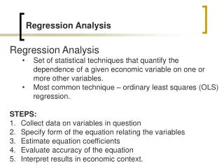
5. 3.2 Introduction to Regression Analysis • Regression is a statistical method for estimating the parameters of an equation (intercept and slopes) • The coefficients (intercept and slopes) are estimated by: • Minimizing the sum of squared distances between the actual values of the dependent variable and the estimated values of the dependent variable

6. 3.2 Introduction to Regression Analysis • Regression can estimate a simple equation with one independent variable, more than one independent variable and more than one dependent variable (simultaneous equation systems) • Y = f(X) • Y = f(X1, X2, …, Xn) • Y = f(X1, X2, …, Xn) and Z = f(Y) • The coefficients (intercept and slopes) are estimated by: • Minimizing the sum of squared distances between the actual values of the dependent variable and the estimated values of the dependent variable

7. 3.2 Introduction to Regression Analysis • Now we add an error term where ε and η are regression error terms. These are stochastic equations as the hypothesized relationship contains randomness: • Y = f(X) + ε • Y = f(X1, X2, …, Xn) + ε • Y = f(X1, X2, …, Xn) + ε (example of PRPM(T)) Z = f(Y) + η • The coefficients (intercept and slopes) are estimated by: • Minimizing the sum of squared distances (squared errors) between the actual values of the dependent variable and the estimated values of the dependent variable

8. 3.2 Introduction to Regression Analysis • The statistical specification of these models are: • Y = a0 + a1 X + ε • Y = a0 + a1 X1 + a2 X2 + … + an Xn + ε • Y = a0 + a1 X1 + a2 X2 + … + an Xn + ε Z = b0 + b1 Y + η (example of PRPM(T) for as system) • The coefficients, i.e., intercept and slopes, or a’s and b’s above are parameters that regression analysis estimates. In the process the regression analysis also estimates the error term(s), namely ε and η.

9. 3.2 Introduction to Regression Analysis • Stochastic v. deterministic graphs and models • Review error term, actual Y versus predicted Y, on stochastic graph for t = 1, …,4

10. 3.2 Introduction to Regression Analysis • Regression analysis estimates the hypothesized relation between the dependent variable(s) and independent variable(s). • The inference of causation that Y is a function of X comes from the theory that lead to the specification of the model. • Correlation measures the strength of the potential linear relation between two variables.

11. 3.3 Diagnostics of Least Squares Estimation • Diagnostics: • Comport with expectations from theory • Slope on price in sales model negative? • Statistical significance of the estimated parameters • Statistical significance / fit of the entire estimated model • Distribution of the error term: Normal? Test with Jarque Bera statistic

12. 3.3 Diagnostics of Least Squares Estimation • Use T distribution to test significance of estimated parameters (intercept and slopes): Y = a0 + a1 X1 + a2 X2 + … + an Xn + ε • T distribution is the ratio of a normal to a chi square distributed variable (e.g., slope / standard error of slope) • T has a zero mean and thicker tails than normal • Tests to see if estimate is different from zero • Choose significance level; usually 5% or less; minimum strength of test from experience is 10%

13. 3.3 Diagnostics of Least Squares Estimation • The Coefficient of Determination: R2 • Is a measure of the percent of the variation in the dependent variable that is explained by the independent variable • If a simple regression, R is the correlation coefficient • Ranges from 0 to 3.0 • Derivation of R2: 3. Graphically 2. Mathematically

14. 3.3 Diagnostics of Least Squares Estimation • The F Statistic: • A test of the significance of R2 and the significance of the entire regression • Ratio of two variances is F distributed • Note that R2 is a ratio of the explained sum of squares to the total sum of squares

15. 3.5 Practicuum in Regression Using EXCEL See Class Notes