The General Linear Model (for dummies…)
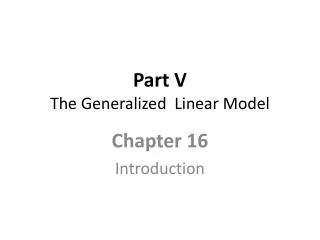
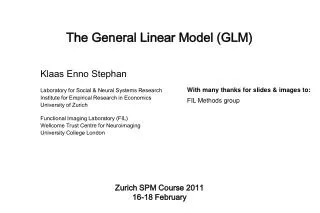
The General Linear Model (for dummies…). Carmen Tur and Ashwani Jha 2009. Overview of SPM. Statistical parametric map (SPM). Design matrix. Image time-series. Kernel. Realignment. Smoothing. General linear model. Gaussian field theory. Statistical inference. Normalisation. p <0.05.


The General Linear Model (for dummies…)
E N D
Presentation Transcript
The General Linear Model (for dummies…) Carmen Tur and Ashwani Jha 2009
Overview of SPM Statistical parametric map (SPM) Design matrix Image time-series Kernel Realignment Smoothing General linear model Gaussian field theory Statistical inference Normalisation p <0.05 Template Parameter estimates
What is the GLM? • It is a model (ie equation) • It provides a framework that allows us to make refined statistical inferences taking into account: • the (preprocessed) 3D MRI images • time information (BOLD time series) • user defined experimental conditions • neurobiologically based priors (HRF) • technical / noise corrections
Data Collect Data Y X How does work? • By creating a linear model:
Collect Data Generate model How does work? • By creating a linear model: Data Y X Y=bx + c
N Collect Data å 2 e = minimum t = t 1 Generate model Fit model How does work? • By creating a linear model: Data Y e X Y=0.99x + 12 + e
Collect Data Generate model Fit model Test model How does work? • By creating a linear model: Data Y e X Y=0.99x + 12 + e
GLM matrix format • But GLM works with lists of numbers (matrices) Y = 0.99x + 12 + e Y = β1X1 + C + e 5.9 1 2 15.0 2 0 18.4 3 5 12.3 4 4 24.7 5 8 23.2 6 8 19.3 7 0 13.6 8 9 26.1 9 1 21.6 10 5 31.7 11 2
GLM matrix format • But GLM works with lists of numbers (matrices) Y = 0.99x + 12 + e Y = β1X1 + β2X2 + C + e 5.9 1 2 15.0 2 2 18.4 3 5 12.3 4 5 24.7 5 5 23.2 6 2 19.3 7 2 13.6 8 5 26.1 9 5 21.6 10 5 31.7 11 2 sphericity assumption We need to put this in… (data Y, and design matrix Xs) ‘non-linear’
GLM matrix format X + y =
A very simple fMRI experiment One session Passive word listening versus rest 7 cycles of rest and listening Blocks of 6 scans with 7 sec TR Stimulus function Question: Is there a change in the BOLD response between listening and rest?
A closer look at the data (Y)… Time Time BOLD signal Look at each voxel over time (mass univariate)
error = + + 1 2 Time e x1 x2 The rest of the model… Instead of C BOLD signal
The GLM matrix format = + X y
…easy! • How to solve the model (parameter estimation) • Assumptions (sphericity of error)
N å 2 e = minimum t = t 1 Solving the GLM (finding ) • Actually try to estimate • ‘best’ has lowest overall error ie the sum of squares of the error: • But how does this apply to GLM, where X is a matrix… ^ ^ e Y=0.99x + 12 + e
…need to geometrically visualise the GLM in N dimensions y x1 x2 ^ = + N ^
…need to geometrically visualise the GLM y x1 x2 ^ + = N=3 x2 Design space defined by y = X What about the actual data y? ^ ^ x1
…need to geometrically visualise the GLM y x1 x2 ^ + = N=3 y x2 Design space defined by y = X ^ ^ x1
ˆ = b ˆ y X Once again in 3D.. • The design (X) can predict the data values (y) in the design space. • The actual data y, usually lies outside this space. • The ‘error’ is difference. y ^ e x2 x1 Design space defined by X
N å 2 e = minimum t = t 1 ˆ = b ˆ y X Solving the GLM (finding ) – ordinary least squares (OLS) • To find minimum error: • e has to be orthogonal to design space (X). “Project data onto model” • ie: XTe = 0 XT(y - X) = 0 XTy = XTX y e x2 x1 Design space defined by X
Assuming sphericity • We assume that the error has: • a mean of 0, • is normally distributed • is independent (does not correlate with itself) =
Assuming sphericity • We assume that the error has: • a mean of 0, • is normally distributed • is independent (does not correlate with itself) = x
Half-way re-cap… GLM Solution Ordinary least squares estimation (OLS) (assuming i.i.d. error): = + y X
GLM Methods for dummies 2009-10 London, 4th November 2009 II part Carmen Tur
Problems of this model HRF Neural stimulus time Neural stimulus hemodynamic response I. BOLD responses have a delayed and dispersed form expected BOLD response Hemodynamic Response Function: This is the expected BOLD signal if a neural stimulus takes place expected BOLD response = input function impulse response function (HRF)
Problems of this model Solution: CONVOLUTION I. BOLD responses have a delayed and dispersed form HRF Transform neural stimuli function into a expected BOLD signal with a canonical hemodynamic response function (HRF)
Problems of this model II. The BOLD signal includes substantial amounts of low-frequency noise WHY? Multifactorial: biorhythms, coil heating, etc… HOW MAY OUR DATA LOOK LIKE? Real data Predicted response, NOT taking into account low-frequency drift Intensity Of BOLD signal Time
Problems of this model II. The BOLD signal includes substantial amounts of low-frequency noise Solution: HIGH PASS FILTERING discrete cosine transform (DCT) set
Interim summary: GLM so far… • Acquisition of our data (Y) • Design our matrix (X) • Assumptions of GLM • Correction for BOLD signal shape: convolution • Cleaning of our data of low-frequency noise • Estimation of βs • But our βs may still be wrong! Why? • Checkup of the error… • Are all the assumptions of the error satisfied? STEPS so far…
Problems of this model e 0 0 t It should be… III. The data are serially correlated Temporal autocorrelation: in y = Xβ + e over time e e in time t is correlated with e in time t-1 t It is…
Problems of this model III. The data are serially correlated Temporal autocorrelation: in y = Xβ + e over time WHY? Multifactorial…
Problems of this model III. The data are serially correlated Temporal autocorrelation: in y = Xβ + e over time et= aet-1 + ε (assuming ε ~ N(0,σ2I)) Autoregressive model autocovariance function in other words: the covariance of error at time t (et) and error at time t-1 (et-1) is not zero
Problems of this model III. The data are serially correlated Temporal autocorrelation: in y = Xβ + e over time et= aet-1 + ε (assuming ε ~ N(0,σ2I)) Autoregressive model et -1= aet-2 + ε et -2= aet-3 + ε … et= aet-1 + ε et=a (aet-2 + ε) + ε et=a2et-2 + aε + ε et=a2(aet-3 + ε) + aε + ε et=a3et-3 + a2ε + aε + ε … But ais a number between 0 and 1
Problems of this model in other words: the covariance of error at time t (et) and error at time t-1 (et-1) is not zero time (scans) ERROR: Covariance matrix 1 2 3 4 5 6 7 8 9 10 1 2 3 4 5 6 7 8 9 10 time (scans)
Problems of this model III. The data are serially correlated Temporal autocorrelation: in y = Xβ + e over time et= aet-1 + ε (assuming ε ~ N(0,σ2I)) Autoregressive model autocovariance function in other words: the covariance of error at time t (et) and error at time t-1 (et-1) is not zero This violates the assumption of the error e ~ N (0, σ2I)
Problems of this model III. The data are serially correlated Solution: 1. Use an enhanced noise model with hyperparameters for multiple error covariance components It should be… It is… et= ε et= aet-1 + ε et= aet-1 + ε ? Or, if you wish et= ε a ≠ 0 But…a? a = 0
Problems of this model III. The data are serially correlated Solution: 1. Use an enhanced noise model with hyperparameters for multiple error covariance components We would like to know covariance (a, autocovariance) of error But we can only estimate it: V V = ΣλiQ i V = λ1Q1 + λ2Q 2 λ1 and λ2: hyperparameters Q1 and Q2: multiple error covariance components It should be… It is… et= aet-1 + ε et= aet-1 + ε ? et= ε a = 0 a ≠ 0 But…a?
Problems of this model III. The data are serially correlated Solution: 1. Use an enhanced noise model with hyperparameters for multiple error covariance components 2. Use estimated autocorrelation to specify filter matrix W for whitening the data et= aet-1 + ε(assuming ε ~ N(0,σ2I)) WY = WXβ + We
Other problems – Physiological confounds • head movements • arterial pulsations (particularly bad in brain stem) • breathing • eye blinks (visual cortex) • adaptation affects, fatigue, fluctuations in concentration, etc.
Other problems – Correlated regressors Example: y = x1β1 + x2β2 + e When there is high (but not perfect) correlation between regressors, parameters can be estimated… But the estimates will be inefficiently estimated (ie highly variable)
Other problems – Variability in the HRF • HRF varies substantially across voxels and subjects • For example, latency can differ by ± 1 second • Solution: MULTIPLE BASIS FUNCTIONS (another talk) HRF could be understood as a linear combination of A, B and C A B C
Ways to improve the model Model everything globalactivity or movement Important to model all known variables, even if not experimentally interesting: effects-of-interest (the regressors we are actually interested in) + head movement, block and subject effects… conditions: effects of interest subjects • Minimise residual error variance
How to make inferences REMEMBER!! • The aim of modelling the measured data was to make inferences about effects of interest • Contrasts allow us to make such inferences • How? T-tests and F-tests Another talk!!!
SUMMARY Using an easy example...
Given data (image voxel, y) Y= X. β+ ε
Different (rigid and known) predictors (regressors, design matrix, X) Y= X. β+ ε Time x6 x5 x4 x3 x2 x1
Fitting our models into our data (estimation of parameters, β) Y= X. β+ ε Y= X. β+ ε x1 x2 x3 x4 x5 x6
Fitting our models into our data (estimation of parameters, β) HOW? Y= X. β+ ε Minimising residual error variance