Download
1 / 51
520 likes | 681 Views
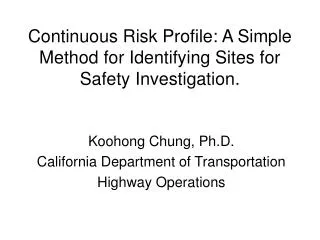
Continuous Risk Profile: A Simple Method for Identifying Sites for Safety Investigation. Koohong Chung, Ph.D. California Department of Transportation Highway Operations. Outline. 2. Continuous Risk Profile . 3. Findings. 1. Motivation and Background. 4. Discussion . 5. Concluding Remarks .

E N D
Continuous Risk Profile: A Simple Method for Identifying Sites for Safety Investigation. Koohong Chung, Ph.D. California Department of Transportation Highway Operations
Outline 2. Continuous Risk Profile 3. Findings 1. Motivation and Background 4. Discussion 5. Concluding Remarks
“Sliding Moving Window” Approach 1. Motivation and Background 0.2 mile roadway the number of collision with the window the reference value
“Sliding Moving Window” Approach 1. Motivation and Background 0.2 mile roadway the number of collision with the window < 0.01 mile the reference value slide the window by small increment of 0.1 mile and repeat the same analysis
“Sliding Moving Window” Approach 1. Motivation and Background 0.2 mile roadway the number of collision with the window > the reference value The site will be reported it to Table-C or Wet Table-C and move the window to the next 0.2 mile segment
1. Motivation and Background A. Identify sites that are adjacent to each other as one site Task Force (2002) conducted survey among 44 safety engineers B. High false positive rate for both Table-C and Wet Table-C
Pattern I: Collision causative factor can reside outside of 0.2 mile window. 1. Motivation and Background Direction of traffic
Pattern II: Collisions can accompany secondary collisions in the vicinity. 1. Motivation and Background
The collision data on freeways were often spatially correlated. 1. Motivation and Background Reference Rate Direction of traffic
2. Continuous Risk Profile A(d) B(d) Cumulative number of Collisions Direction of traffic
2. Continuous Risk Profile Rescaled Cumulative Collision Count Curve (I-880 Northbound, Alameda County, California, 2003)
CRP M(d) = 2. Continuous Risk Profile For and Where Dstart < Dend l = increment f(d) = A(d) – B(d-do) d0 = beginning postmile dend = ending postmile 2L = size of the moving average and K, are integers
CRP M(d) = 2. Continuous Risk Profile For A Method for Generating a Continuous Risk Profile for Highway Collisions (2007) Chung and Ragland and Where To be Determined , (working paper) Chung, Ragland and Madanat Dstart < Dend l = increment f(d) = A(d) – B(d-do) d0 = beginning postmile dend = ending postmile 2L = size of the moving average and K, are integers
2. Continuous Risk Profile postmile By dividing the above CRP by AADT, the unit can be converted to number of collisions per vehicle miles.
Comment from hydraulic division We were thinking that a plot like these presented to Hydraulics prior to a major rehabilitation project would be ideal in assisting us evaluate and upgrade drainage at the high accident locations as necessary. …Could I encourage you to have a discussion at the end of your report recommending that Caltrans generate such plots? It (CRP plot) would help us out immeasurably during design. -Joseph Peterson, Office Chief ,District 4 Hydraulic-
3. Findings Findings 1: CRP can be used to identify freeway sites that display high collision rate only under wet pavement condition.
DRY WET WET ONLY
DRY “Identification of High Collision Concentration Locations Under Wet Weather Conditions”, Hwang, Chung, Ragland, and Chan WET WET ONLY
3. Findings Findings 2: CRP are reproducible over the years and can proactively monitor traffic collisions.
3. Findings Findings 3: CRP plots can be used to capture the “spill over benefit”.
Project Completed in 2001 Postmile
Spillover Benefit Postmile
3. Findings Findings 4: Using CRP, you can save time in site investigation.
Access OFF ON 2003 2002 2001 2000 1999 Direction of Traffic PM 18.1
PM 17.887 PM 18.141 PM 18.3
Accidents Rate (Accidents/Mile) (SR-91W) 4 Times Higher 4 Times Higher
Accidents Data Analysis (PDO) 2 Times Higher
Accidents Data Analysis (INJURY) 3 Times Higher
Due to the inclined freeway, drivers tend to accelerate
1) Inclined On-Ramp 2) Heavy vegetations
Map of HCCL (SR-91 W) 1) Inclined On-Ramp 2) Heavy vegetations
3. Findings More Findings: “Comparison of Collisions on HOV facilities with Limited and Continuous Access during Peak Hours”, Jang, Chung, Ragland, and Chan “Identification of High Collision Concentration Locations Under Wet Weather Conditions”, Hwang, Chung, Ragland, and Chan
4. Discussion Highways Intersections YES (SafetyAnalyst) Ramp
4. Discussion LOSS -IV +1.5 б LOSS -III SPF Accidents Per Mile Per Year LOSS -II -1.5 б LOSS -I AADT (“Level of Service of Safety”, Kononov and Allery)
4. Discussion LOSS -IV +1.5 б LOSS -III SPF Accidents Per Mile Per Year LOSS -II -1.5 б LOSS -I AADT (“Level of Service of Safety”, Kononov and Allery)
4. Discussion “.. ML estimation of both Poisson and negative binomial regression typically requires independent observations. This assumption will often not be true in time-series data, and Poisson and negative binomial regression are then problematic.” “The Analysis of Count data: overdispersion and autocorrelation”, Barron
4. Discussion biased SPF Unbiased SPF Accidents Per Mile Per Year biased SPF AADT
Spatial correlation is not an issue in constructing CRP 5. Concluding Remark CRP is simple to use and provides overview of collision rates of extended segment of freeways over the years. CRP can proactively monitor traffic collision rates. CRP can identify sites that display high collision rates only under certain condition. (ex: wet hot spots) CRP can be used to capture “spill over benefit” of countermeasure.
In future research, 5. Concluding Remark I. Continue exploring different areas where CRP can be used. II. Friendly interface CALTRANS III. Expand CRP approach for CALTRANS intersections and ramp.