Download
1 / 21
230 likes | 417 Views
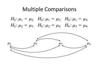
IV Multiple Comparisons A. Contrast Among Population Means ( i ) 1. A contrast among population means is a difference among the means with appropriate algebraic sign. pairwise contrast: nonpairwise contrast:. 2. Contrasts are defined by a set of underlying

E N D
IV Multiple Comparisons A. Contrast Among Population Means (i) 1. A contrast among population means is a difference among the means with appropriate algebraic sign. pairwise contrast: nonpairwise contrast:
2. Contrasts are defined by a set of underlying coefficients (cj ) with the following characteristics: The sum of the coefficients must equal zero, cj ≠ 0 for some j For convenience (to put all contrasts on the same measurement scale), coefficients are chosen so that
3. Pairwise contrast for means 1 and 2, where c1 = 1 and c2 = –1 4. Nonpairwise contrast for means 1, 2, and 3, where c1 = 1, c2 = –1/2, and c3 = –1/2
5. Pairwise contrast: all of the coefficients except two are equal to 0. 6. Nonpairwise contrast: at least three coefficients are not equal to 0. 7. A contrast among sample means, denoted by is a difference among the sample means with appropriate algebraic sign.
V Fisher-Hayter Multiple Comparison Test A. Characteristics of the Test 1. The test uses a two-step procedure. The first steps consists of testing the omnibus null hypothesis using an F statistic. 2. If the omnibus test is significant, the Fisher-Hayter statistic is used to test all pairwise contrasts among the p means.
B. Fisher-Hayter Test Statistic where and are means of random samples from normal populations, MSWG is the denominator of the F statistic from an ANOVA, and nj and njare the sizes of the samples used to compute the sample means.
1. Reject H0:j = jif |qFH| statistic exceeds or equals the critical value, , from the Studentized range table (Appendix Table D.10). C. Computational Example Using the Weight- Loss Data 1. Step 1. Test the omnibus null hypothesis 2. Step 2. Because F is significant, test all pairwise contrasts using qFH.
D. Assumptions of the Fisher-Hayter Test 1. Random sampling or random assignment of participants to the treatment levels 2. The j = 1, . . . , p populations are normally distributed. 3. The variances of the j = 1, . . . , p populations are equal.
VI Scheffé Multiple Comparison Test and Confidence Interval A. Characteristics of the Test 1. The test does not require a significant omnibus test. 2. Can test both pairwise and nonpairwise contrasts and construct confidence intervals. 3. The test is less powerful than the Fisher-Hayter test for pairwise contrasts.
B. Scheffé Test Statistic where c1, c2, . . . , cp are coefficient that define a contrast, , . . . , are sample means, MSWG is the denominator of the ANOVA F statistic, and n1, n2, . . . , np are the sizes of the samples used to compute the sample means.
1. Reject a null hypothesis for a contrastif the FS statistic exceeds or equals the critical value, is obtained from the F table (Appendix Table D.5). C. Computational Example Using the Weight- Loss Data 1. Critical value is
E. Assumptions of the Scheffé Test and Confidence Interval 1. Random sampling or random assignment of participants to the treatment levels 2. The j = 1, . . . , p populations are normally distributed. 3. The variances of the j = 1, . . . , p populations are equal.
F. Comparison of Fisher-Hayter and Scheffé Tests 1. The Fisher-Hayter test controls the Type I error at for the collection of all pairwise contrasts. 2. The Scheffé test controls the Type I error at for the collection of all pairwise and nonpairwise contrasts. 3. The Scheffé statistic can be used to construct confidence intervals.
VII Practical Significance A. Omega Squared 1. Omega squared estimates the proportion of the population variance in the dependent variable that is accounted for by the p treatments levels. 2. Computational formula
3. Cohen’s guidelines for interpreting omega squared 4. Computational example for the weight-loss data
B. Hedges’s g Statistic 1. g is used to assess the effect size of contrasts 2. Computational example for the weight-loss data