Download
1 / 33
350 likes | 499 Views
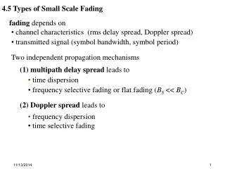
4.5 Types of Small Scale Fading. fading depends on channel characteristics (rms delay spread, Doppler spread) transmitted signal (symbol bandwidth, symbol period) Two independent propagation mechanisms (1) multipath delay spread leads to time dispersion

E N D
4.5 Types of Small Scale Fading • fading depends on • channel characteristics (rms delay spread, Doppler spread) • transmitted signal (symbol bandwidth, symbol period) • Two independent propagation mechanisms • (1) multipath delay spread leads to • time dispersion • frequency selective fading or flat fading (BS << BC) • (2) Doppler spread leads to • frequency dispersion • time selective fading
(1) multipath time-delay spread = rms delay spread BC = coherence bandwidth BS < BC TS > BS > BC TS < Frequency Selective Fade Flat Fade (2) Doppler spread BD = Doppler spread TC = coherence time TS > TC BS < BD TS < TC BS > BD Slow Fade Fast Fade Small Scale Fading BS = signal bandwidth, TS = symbol period = BS-1 High Doppler Spread
4.5.1.1 Flat Fading (FF) channel occurs when BC >> BS & TS >> • channel response has constant gain & linear phase • channel’s multipath structure preserves signal’s spectral • characteristics • time varying received signal strength due to gain fluctuations MPCs • - amplitude changes in received signal, r(t) due to gain fluctuations • - spectrum of r(t) transmission is preserved • typically cause deep fades compared to non-fading channel • - in a deep fade,may require 20dB-30dB transmit power for low BER • 4.5.1 Fading Due to Multipath Time Delay Spread • time dispersion from multipath causes either • flat fading • frequency selective fading
Channels Complex Envelope,hb(t,) is approximated as having no • excess delay • a single delta function with = 0 • Distribution of instantaneous gain for FF channels is an importantRF design issue • Rayleigh Distribution is the most common amplitude distribution • Rayleigh Flat Fading Model assumes channel induces time • varying amplitude according to Rayleigh Distribution
time response s(t) h(t,) r(t) 0 TS 0 TS+, 0 channel H(f) R(f) frequency response S(f) fc fc fc Flat Fading Time & Frequency Response assume << Ts
s(t) r(t) Channel 4.5.1.2 Frequency Selective Fading (FSF) • FF Bandwidth = Channel Bandwidth over which signals experience • constant gain & linear phase • statistical variation in amplitude • if BS>>FF bandwidth s(t) experiences FSF • channel impulse response has multipath delay spread > TS • r(t) is distorted & includes multiple versions of transmitted • waveform that are • - attenuated (faded) • - delayed in time • FSF is due to time-dispersion of transmitted symbols within channel • inter-symbol interference (ISI) induced by channel • different frequency components of R(f) have different gains
FSF also known as wideband channelsBS > bandwidth of channel’s impulse response • difficult to model each multipath signal must be modeled • channel must be considered to be a linear filter • wideband multipath measurements are used to develop multipath • models • Small Scale FSF Models used for analysis of mobile communications • 1. Statistical Impulse Response Models • 2-ray Rayleigh Fading model • - models impulse response as 2 delta functions () • - ’s independently fade and have sufficient time delay • between them to induce FSF • 2. Computer Generated Impulse Responses • 3. Measured Impulse Responses
s(t) h(t,) r(t) time response 0 0 TS 0 TS TS+ channel frequency response S(f) H(f) R(f) fc fc fc Frequency Selective Fading Time & Frequency Response
FSF fading occurs when BS> BCand TS < • Common Rules of thumb • Channel is FF if TS 10 • Channel is FSF if TS < 10 • actual values depend on modulation technique • time-delay spread has significant impact on BER • FSF channel - different gain for different spectral components of S(f) • S(f) = spectrum of transmitted signal s(t) • BS = bandwidth of transmitted signal s(t) • FSF caused by MPC delays which exceed TS = BS-1 • time varying channel gain & phase over spectrum of s(t) • results in distorted signal r(t)
FSF Channel model for large scale effects in complex phasor notation L ~ ~ ~ å = a - t x ( t ) s ( t ) l l = l 1 l = relative delay of lth path • a signal’s MPCs may have different path lengths • complex gain assumed constant practically, true if receiver & • transmitter are stationary channel impulse response becomes channel response is time invariant but frequency dependent = complex gains
2.4 2.2 2.0 1.8 1.6 1.4 1.2 1.0 0.8 0.6 0.4 0.2 0.0 2 = -j 2 = 0.5 2 = j/2 amplitude response -0.4 -0.2 0.0 0.2 0.4 frequency (sample rates) e.g. assume 2-ray FSF Channel with impulse response: • 2 = relative delay of 2nd path • simulate channel digitally with sample period = Ts = 2 (fs = sampling • frequency) • channels frequency response will vary for different values of α2
4.5.2 Fading Effects Due to Doppler Spread • fading is affected by s(t)’s rate of change vs channel’s rate of change • (i) fast fading channel: channel impulse response changes rapidly during • symbol period TS • (ii) slow fading channel: channel impulse response changes slowly • during TS 4.5.2.1 Fast Fading - results in distorted r(t) Fast Fading assumes all reflected paths have equal lengths& delays • Fast Fading occurs when • (i) symbol period is longer than coherence time: TS > TC and • (ii) symbol bandwidth is less than Doppler Spread: BS < BD • time-selective fading:BD causes frequency dispersion • signal distortion from fast fading increases with larger BD
4.5.2.2 Slow Fading Slow Fading occurs when (i) symbol period is much less than coherence time: TS << TC and (ii) symbol bandwidth is much greater than Doppler Spread: BS >> BD • channel assumed static over one or more symbol periods, TS • Fast fading or Slow fading determined by relationship of TS to • (i) velocity of mobile terminals and • (ii) velocity of objects in the channel • deals with time rate of change of channel & signal (small scale • fading) • does not deal with path loss models (large scale fading)
channel impulse response is time varying h(t,τ) = α(t)δ(t) • α(t) is time varying received signal strength is also time varying Time-selective Channel • Power Spectrum of received signal = power spectra of transmitted • signal convolved with power spectra of fading process • multiplication in time domain = convolution in frequency domain Sr(f) = S(f) Ss(f) • Sr(f) = power spectrum of received signal • S(f) = power spectrum of fading process • Ss(f) = power spectrum of transmitted signal
1.0 0.8 0.6 0.4 0.2 0.0 doppler spread spectrum original spectrum Frequency Response -2000 -1000 0 1000 2000 Frequency H(z) • Nominal transmitted spectrum power spectrum of fading process original spectrum vs doppler spread spectrum • Assume doppler spectrum 20% of signal bandwidth B3dB 5fm • fm = maximum doppler shift • B3dB = 3dB bandwidth of nominal spectrum
Flat Fading Channel Response: time selective & frequency flat L ~ ~ ~ å = a - t x ( t ) s ( t ) l l = l 1 time varying channel impulse response Frequency Selective Channel: large scale effects l = relative delay of lth path = complex gains time invariant but frequency dependent channel response
TS = Transmitted Symbol Period TS Flat Slow Fade Flat Fast Fade Frequency Selective Fast Fade Frequency Selective Slow Fade TC TS BS = Transmitted Baseband Signal BW BS Frequency Selective Fast Fade Frequency Selective Slow Fade BC Flat Slow Fade Flat Fast Fade BD BS
4.5.3 General Channels (i) flat-flat channel: neither frequency or time varying • (ii) time selective and frequency selective channel • MPCs of signal have different lengths frequency selective fading • interaction of MPCs generated locally time-varying fading received signal given as time varying channel impulse response is • channel model includes large and small scale effects • h(t,) is for finite number of signal paths • - represents continuum of MPC with arbitrarily small differences • - both time selective & frequency selective
time varying frequency response (transfer function) given by H(t,f) = F[ h(t,τ)] • received signal = channel response transmitted signal • with either discrete or continuum number of MPCs
e.g. time varying impulse response 0.35 0.30 0.25 0.20 0.15 0.10 0.05 0.00 25 20 15 10 5 0 spectrum time (ms) consider 400 300 200 100 0 -100 -200 -300 -400 kHz • where {αi(t)} are independent Rayleigh Processes • at time t = t0 Fourier Transform reveals power spectrum • different frequencies with nulls and strong responses vary with time
4.6 Rayleigh & Ricean Distributions • 4.6.1 Rayleigh Fading Distributions • in mobile RF channels commonly used to model describe statistical time • varying nature of • (i) received envelope for FF signal • (ii) envelope of a single MPC • envelope sum of 2 quadrature Gaussian noise signals obeys Rayleigh • distribution 10 5 0 -5 -10 -15 -20 -25 Rx Speed ≈ 120km/hr signal level (dB about rms) 0 50 100 (ms) λ/2 Rayleigh distributed signal vs time
Multipath Reflections due to local objects arrive at stationary receiver • nthpath has electric field strength En& relative phaseθn • complex phasor of N signal reflections given by ∆ = • Ẽ is a RV representing effects of multipath channel Ẽ = small changes in path length large changes in phase ∆x = difference in path length ∆ = change in phase e.g. fc = 2.4GHz ( 0.125m) ∆ = 50.26 ∆x
= Zr +jZi Consider mean of nth component of Ẽ , denoted as Enexp(jθn) E[Enexp(jθn)] = E[En] = E[En] E[exp(jθn)] = E[En] (0+0) = 0 • Model for complex channel envelope is Σ iid complex RVs • Central Limit Theorem: for large N Ẽ becomes Gaussian distribution where Zr and Ziare real Gaussian random variables thus E[Ẽ] = 0 and Ẽ is a 0-mean Gaussian RV
E[|Ẽ|2] = (equals 0 for all n ≠ m) = E = E E Considervariance (power) in Ẽ given by mean square value • θn- θmis the difference of 2 random phases = random phase • by symmetry power is equally distributed between real & imaginary • parts of Ẽ • P0 = average receive power
Define the amplitude of the complex envelope, Ẽ as R = PDF of amplitude is determined by changing variables of f ( z ) z r r Complex Envelop, Ẽ has 0-mean Zr & Zi have Gaussian PDF 2 = P0/2 for Zrand Zi
0 ≤ r ≤ p(r) = (4.49) r < 0 0.6065 p(r) p(r)= Pr[r = ] = 0 2 3 4 5 r Rayleigh PDF given by = rms value of received voltage before envelope detection 2 = time average power of received signal before envelope detection Received Signal Envelope Voltage
(4.50) Mean Value of Rayleigh Distributed Signal rmean = E[r] = (4.51) Variance of Rayleigh Distribution represents ac power in signal envelope 2r = E[r2] – E2[r] = P(R) = Pr[r R] = (4.52) = • Rayleigh CDF • probability that received signal’s envelope doesn’t exceed specific value, R
Envelope’s rms Value is the square root of mean square or r = = = = rms voltage of original signal prior to envelope detection Median Value of r is found by (4.53) rmedian = 1.177 (4.54) = 1.414
1 0.1 0.01 10-3 10-4 -40 -30 -20 -10 0 10 amplitude 20log10(R/Rrms) Pr (r < R) • Conceptually, each location corresponds to different set of {n} • deep fades >20dB (R < 0.1Rrms)occur only about 1% • wide variation in received signal strength due to local reflections • if received signal were measured from a number of stationary locations • power measurements would show Rayleigh distribution Rayleigh Distribution Graph
Rayleigh Fading Signal • mean & median differ by only 0.07635 (0.55dB) • in practice - median is often used • - fading data usually consists of field measurements & a particular • distribution cannot be assumed • - use of median allows easy comparison of different fading • distributions with widely varying means
4.6.2 Ricean Fading Distributions • if signal has dominant stationary component (LOS path) small scale • fading envelopehas Ricean Distribution • random MPCs arrive at different angles & are superimposed on dominant • signal • envelope detector output yields DC component + random MPCs • Ricean distribution is result of dominant signal arriving with weaker MPCs • as dominant component fades Ricean distribution degenerates to • Rayleigh distribution • composite signal resembles noise signal with envelope that is Rayleigh • same as in the case of sine wave detection in thermal noise
A ≥ 0 , r ≥ 0 p(r) = (4.55) r < 0 p(r) K = - dB (4.56) K = 6 dB received signal envelope voltage K = K (dB) = r Ricean PDF A = peak amplitude of dominant signal 0() = modified Bessel function of the 1st kind & zero order • Ricean Distribution often described in terms of Ricean FactorK • K = ratio of deterministic signal power to multipath variance • as dominate path attenuates A grows small • Ricean distribution degenerates to Rayleigh
Ricean Fading Pr (r < R) 1 0.1 0.01 10-3 10-4 K = 0 (Rayleigh) K=5dB K=10dB K=13dB -40 -30 -20 -10 0 10 amplitude 20log10(R/Rrms) probability of deep fades reduced as K grows