Image Visualization
Understand image processing basics like contrast enhancement and histogram equalization, learn about smoothing to remove noise, and explore frequency domain techniques to enhance image quality.

Image Visualization
E N D
Presentation Transcript
Outline • 9.1. Image Data Representation • 9.2. Image Processing and Visualization • 9.3. Basic Imaging Algorithms • Contrast Enhancement • Histogram Equalization • Gaussian Smoothing • Edge Detection • 9.4. Shape Representation and Analysis • Segmentation • Connected Components • Morphological Operations • Distance Transforms • Skeletonization
Image Data Representation What is an image? • An image is a well-behaved uniform dataset. • An image is a two-dimensional array, or matrix of pixels, e.g., bitmaps, pixmaps, RGB images • A pixel is square-shaped • A pixel has a constant value over the entire pixel surface • The value is typically encoded in 8 bits integer
Image Processing and Visualization • Image processing follows the visualization pipeline, e.g., image contrast enhancement following the rendering operation • Image processing may also follow every step of the visualization pipeline
Basic Image Processing • Image enhancement operation is to apply a transfer function on the pixel luminance values • Transfer function is usually based on image histogram analysis • High-slope function enhance image contrast • Low-slope function attenuate the contrast.
(Continued) Image Visualization Chap. 9 November 12, 2009
Basic Image Processing • The basic image processing is the contrast enhancement through applying a transfer function
Image Enhancement Linear Transfer Non-linear Transfer
Histogram Equalization • All luminance values covers the same number of pixels • Histogram equalization method is to compute a transfer function such as the resulted image has a near-constant histogram
Histogram Equalization • Histogram equalization is a technique for adjusting image intensities to enhance contrast. • In general, a histogram is the estimation of the probability distribution of a particular type of data. • An image histogram is a type of histogram which offers a graphical representation of the tonal distribution of the gray values in a digital image. • By viewing the image’s histogram, we can analyze the frequency of appearance of the different gray levels contained in the image.
Histogram Equalization Original Image After equalization
Smoothing How to remove noise? • Fact: Images are noisy • • Noise is anything in the image that we are not interested in • Noise can be described as rapid variation of high amplitude • Or regions where high-order derivatives of f have large values • Smoothing is often used to reduce noise within an image
Smoothing Noise image After filtering
Fourier Transform • The Fourier Transform is an important image processing tool which is used to decompose an image into its sine and cosine components. • The output of the transformation represents the image in the Fourier or frequency domain, while the input image is the spatial domain equivalent. • In the Fourier domain image, each point represents a particular frequency contained in the spatial domain image.
Spatial Domain Vs Frequency Domain • Spatial Domain (Image Enhancement) • is manipulating or changing an image representing an object in space to enhance the image for a given application. • Techniques are based on direct manipulation of pixels in an image • Used for filtering basics, smoothing filters, sharpening filters, unsharp masking and laplacian • 2. Frequency DomainTechniques are based on modifying the spectral transform of an image • Transform the image to its frequency representation • Perform image processing • Compute inverse transform back to the spatial domain
Frequency Filtering • Computer the Fourier transform F(wx,wy) of f(x,y) • Multiple F by the transfer function Φ to obtain a new function G, e.g., high frequency components are removed or attenuated. • Compute the inverse Fourier transform G-1 to get the filtered version of f
Frequency Filtering • Frequency filter function Φcan be classified into three different types: • Low-pass filter: A low-pass filter is a filter that passes signals with a frequency lower than a certain cutoff frequency and attenuates signals with frequencies higher than the cutoff frequency. • High-pass filter: A high-pass filter is an electronic filter that passes signals with a frequency higher than a certain cutoff frequency and attenuates signals with frequencies lower than the cutoff frequency. • Band-pass filter: A band-pass filter is a device that passes frequencies within a certain range and rejects (attenuates) frequencies outside that range. To remove noise, low-pass filter is used
Gaussian Filter • In image processing, a Gaussian blur (also known as Gaussian smoothing) is the result of blurring an image by a Gaussian function. • It is a widely used effect in graphics software, typically to reduce image noise and reduce detail. • Gaussian smoothing is also used as a pre-processing stage in computer vision algorithms in order to enhance image structures at different scales. • The Gaussian outputs a `weighted average' of each pixel's neighborhood, with the average weighted more towards the value of the central pixels. • This is in contrast to the mean filter's uniformly weighted average. Because of this, a Gaussian provides gentler smoothing and preserves edges better than a similarly sized mean filter. To remove noise, low-pass filter is used
Edge Detection • Edge detection is an image processing technique for finding the boundaries of objects within images. • It works by detecting discontinuities in brightness. Edge detection is used for image segmentation and data extraction in areas such as image processing, computer vision, and machine vision. • Edges are curves that separate image regions of different luminance • The points at which image brightness changes sharply are typically organized into a set of curved line segments termed edges.
Origin of Edges • Edges are caused by a variety of factors surface normal discontinuity depth discontinuity surface color discontinuity illumination discontinuity
Edge Detection Original Image Edge Detection
First Order Derivative Edge Detection Generally, the first order derivative operators are very sensitive to noise and produce thicker edges. a.1) Roberts filtering: diagonal edge gradients, susceptible to fluctations. Gives no information about edge orientation and works best with binary images. a.2) Prewitt filter: The Prewitt operator is a discrete differentiation operator which functions similar to the Sobel operator, by computing the gradient for the image intensity function. Makes use of the maximum directional gradient. As compared to Sobel, the Prewitt masks are simpler to implement but are very sensitive to noise. a.3) Sobel filter: Detects edges are where the gradient magnitude is high.This makes the Sobel edge detector more sensitive to diagonal edge than horizontal and vertical edges.
2nd Order Derivative Edge Detection • If there is a significant spatial change in the second derivative, an edge is detected. • Good on producing thinner edges. • 2nd Order Derivative operators are more sophisticated methods towards automatized edge detection, however, still very noise-sensitive. • As differentiation amplifies noise, smoothing is suggested prior to applying the Laplacians. In that context, typical examples of 2nd order derivative edge detection are the Difference of Gaussian (DOG) and the Laplacian of Gaussian
(Continued) Image Visualization Chap. 9 November 19, 2009
Shape Representation and Analysis Shape Analysis Pipeline
Shape Representation and Analysis • Filtering high-volume, low level datasets into low volume dataset containing high amounts of information • Shape is defined as a compact subset of a given image • Shape is characterized by a boundary and an interior • Shape properties include • geometry (form, aspect ratio, roundness, or squareness) • Topology (type, kind, number) • Texture (luminance, shading)
Segmentation • Segment or classify the image pixels into those belonging to the shape of interest, called foreground pixels, and the remainder, also called background pixels. • Segmentation results in a binary image • Segmentation is related to the operation of selection, i.e., thresholding
Segmentation Find soft tissue Find hard tissue
Connected Components Find non-local properties Algorithm: start from a given foreground pixels, find all foreground pixels that are directly or indirectly neighbored
Morphological Operations To close holes and remove islands in segmented images a: original image b: segmentation c: close holes d: remove island
Introduction • Morphology: a branch of image processing that deals with the form and structure of an object. • Morphological image processing is used to extract image components for representation and description of region shape, such as boundaries, skeletons, and shape of the image.
Structuring Element (Kernel) • Structuring Elements can have varying sizes • Usually, element values are 0,1 and none(!) • Structural Elements have an origin • For thinning, other values are possible • Empty spots in the Structuring Elements are don’t care’s! Box Disc Examples of stucturing elements
Dilation & Erosion • Basic operations • Are dual to each other: • Erosion shrinks foreground, enlarges Background • Dilation enlarges foreground, shrinks background
Erosion • Erosion is the set of all points in the image, where the structuring element “fits into”. • Consider each foreground pixel in the input image • If the structuring element fits in, write a “1” at the origin of the structuring element! • Simple application of pattern matching • Input: • Binary Image (Gray value) • Structuring Element, containing only 1s!
Erosion Operations (cont.) Structuring Element (B) Original image (A) Intersect pixel Center pixel
Erosion Operations (cont.) Result of Erosion Boundary of the “center pixels” where B is inside A
Dilation • Dilation is the set of all points in the image, where the structuring element “touches” the foreground. • Consider each pixel in the input image • If the structuring element touches the foreground image, write a “1” at the origin of the structuring element! • Input: • Binary Image • Structuring Element, containing only 1s!!
Dilation Operations (cont.) Reflection Structuring Element (B) Intersect pixel Center pixel Original image (A)
Dilation Operations (cont.) Result of Dilation Boundary of the “center pixels” where intersects A
Opening & Closing • Important operations • Derived from the fundamental operations • Dilatation • Erosion • Usually applied to binary images, but gray value images are also possible • Opening and closing are dual operations
Morphological Operations • Morphological closing: dilation followed by an erosion • Morphological opening: erosion followed by a dilation operation
Opening • Similar to Erosion • Spot and noise removal • Less destructive • Erosion next dilation • the same structuring element for both operations. • Input: • Binary Image • Structuring Element, containing only 1s!
Opening • erosion followed by a dilation operation • Take the structuring element (SE) and slide it around inside each foreground region. • All pixels which can be covered by the SE with the SE being entirely within the foreground region will be preserved. • All foreground pixels which can not be reached by the structuring element without lapping over the edge of the foreground object will be eroded away!
Opening • Structuring element: 3x3 square
Opening Example • Opening with a 11 pixel diameter disc
Closing • Similar to Dilation • Removal of holes • Tends to enlarge regions, shrink background • Closing is defined as a Dilatation, followed by an Erosion using the same structuring element for both operations. • Dilation next erosion! • Input: • Binary Image • Structuring Element, containing only 1s!
Closing • : dilation followed by an erosion • Take the structuring element (SE) and slide it around outside each foreground region. • All background pixels which can be covered by the SE with the SE being entirely within the background region will be preserved. • All background pixels which can not be reached by the structuring element without lapping over the edge of the foreground object will be turned into a foreground.