Download
1 / 8
110 likes | 466 Views
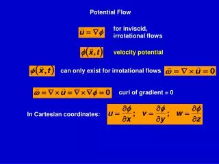
Potential Flow. curl of gradient = 0. In Cartesian coordinates:. for inviscid , irrotational flows. can only exist for irrotational flows. velocity potential. In Cartesian coordinates:. Incompressible flows:. For incompressible, irrotational flows, the governing equation is:.

E N D
Potential Flow curl of gradient = 0 In Cartesian coordinates: for inviscid, irrotational flows can only exist for irrotational flows velocity potential
In Cartesian coordinates: Incompressible flows: For incompressible, irrotational flows, the governing equation is: continuity in terms of the velocity potential: Laplace’s equation
Although incompressibility is not required for a velocity potential to exist, only incompressible, irrotational flows are called Potential Flows The advantage of using a velocity potential, instead of a velocity vector is that one scalar function can contain all three components of velocity vector Potential function - Points of different clusters fall in separate valleys Potential Flows http://today.slac.stanford.edu/images/2009/data-mining.jpg
The stream functionψ is another scalar function that contains all velocity components For 2-D incompressible flows: Continuity equation: is satisfied if Ψis differentiable For 2-D irrotational flows: For incompressible & irrotational 2-D flows, ψ satisfies Laplace’s eq. Therefore, for potential flows, both Φ and ψ satisfy Laplace’s eq.
Partial differential equation -- elliptic Boundary conditions need to be specified around the entire domain b) Specify at normal to boundaries : Neumann boundary condition c) Specify at (any linear combination of a) and b)): Robin boundary condition a) Specify at boundaries : Dirichlet boundary condition Potential Flows
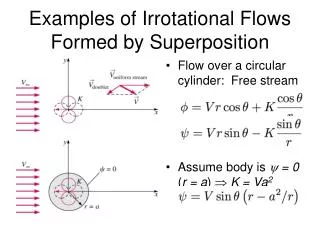
Uniform Flow y u x Examples of Potential Flows
[x,y]=meshgrid(0:.05:2,0:.05:1); fi=0.5*x; contourf(x,y,fi) xlabel('x','FontSize',14); ylabel('y','FontSize',14); title({'Potential Function for ux'},'FontSize',14); colorbar('FontSize',14);
figure psi=-.5*y; contourf(x,y,psi) xlabel('x','FontSize',14); ylabel('y','FontSize',14); title({'Stream Function for -uy'},'FontSize',14); colorbar('FontSize',14);