Download
1 / 64
730 likes | 1.22k Views
MECH 221 FLUID MECHANICS (Fall 06/07) Chapter 7: INVISCID FLOWS. Instructor: Professor C. T. HSU. 7.1 Inviscid Flow. Inviscid flow implies that the viscous effect is negligible. This occurs in the flow domain away from a solid boundary outside the boundary layer at Re .

E N D
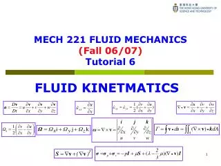
MECH 221 FLUID MECHANICS(Fall 06/07)Chapter 7: INVISCID FLOWS Instructor: Professor C. T. HSU
7.1 Inviscid Flow • Inviscid flow implies that the viscous effect is negligible. This occurs in the flow domain away from a solid boundary outside the boundary layer at Re. • The flows are governed by Euler Equationswhere , v, and p can be functions of r and t .
7.1 Inviscid Flow • On the other hand, if flows are steady but compressible, the governing equation becomeswhere can be a function of r • For compressible flows, the state equation is needed; then, we will require the equation for temperature T also.
7.1 Inviscid Flow • Compressible inviscid flows usually belong to the scope of aerodynamics of high speed flight of aircraft. Here we consider only incompressible inviscid flows. • For incompressible flow, the governing equations reduce to where = constant.
7.1 Inviscid Flow • For steady incompressible flow, the governing eqt reduce further to where = constant. • The equation of motion can be rewrited into • Take the scalar products with dr and integrate from a reference at along an arbitrary streamline =C , leads to since
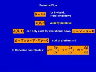
7.1 Inviscid Flow • If the constant (total energy per unit mass) is the same for all streamlines, the path of the integral can be arbitrary, and in the flow domain except inside boundary layers. • Finally, the governing equations for inviscid, irrotational steady flow are • Since is the vorticity , flows with are called irrotational flows.
7.1 Inviscid Flow • Note that the velocity and pressure fields are decoupled. Hence, we can solve the velocity field from the continuity and vorticity equations. Then the pressure field is determined by Bernoulli equation. • A velocity potential exists for irrotational flow, such that, and irrotationality is automatically satisfied.
7.1 Inviscid Flow • The continuity equation becomeswhich is also known as the Laplace equation. • Every potential satisfy this equation. Flows with the existence of potential functions satisfying the Laplace equation are called potential flow.
7.1 Inviscid Flow • The linearity of the governing equation for the flow fields implies that different potential flows can be superposed. • If 1 and 2 are two potential flows, the sum =(1+2) also constitutes a potential flow. We have • However, the pressure cannot be superposed due to the nonlinearity in the Bernoulli equation, i.e.
7.2 2D Potential Flows • If restricted to steady two dimensional potential flow, then the governing equations become • E.g. potential flow past a circular cylinder with D/L <<1 is a 2D potential flow near the middle of the cylinder, where both w component and /z0. U L y x z D
7.2 2D Potential Flows • The 2-D velocity potential function givesand then the continuity equation becomes • The pressure distribution can be determined by the Bernoulli equation,where p is the dynamic pressure
7.2 2D Potential Flows • For 2D potential flows, a stream function (x,y) can also be defined together with (x,y). In Cartisian coordinates, where continuity equation is automatically satisfied, and irrotationality leads to the Laplace equation, • Both Laplace equations are satisfied for a 2D potential flow
and and 7.2 Two-Dimensional Potential Flows • For two-dimensional flows, become: • In a Cartesian coordinate system • In a Cylindrical coordinate system
7.2 Two-Dimensional Potential Flows • Therefore, there exists a stream function such that in the Cartesian coordinate system and in the cylindrical coordinate system. • The transformation between the two coordinate systems
7.2 Two-Dimensional Potential Flows • The potential function and the stream function are conjugate pair of an analytical function in complex variable analysis. The conditions: • These are the Cauchy-Riemann conditions. The analytical property implies that the constant potential line and the constant streamline are orthogonal, i.e., and to imply that .
7.3 Simple 2-D Potential Flows • Uniform Flow • Stagnation Flow • Source (Sink) • Free Vortex
7.3.1 Uniform Flow • For a uniform flow given by , we have • Therefore, • Where the arbitrary integration constants are taken to be zero at the origin. and and
7.3.1 Uniform Flow • This is a simple uniform flow along a single direction.
7.3.2 Stagnation Flow • For a stagnation flow, . Hence, • Therefore,
y x 7.3.2 Stagnation Flow • The flow an incoming far field flow which is perpendicular to the wall, and then turn its direction near the wall • The origin is the stagnation point of the flow. The velocity is zero there.
7.3.3 Source (Sink) • Consider a line source at the origin along the z-direction. The fluid flows radially outward from (or inward toward) the origin. If m denotes the flowrate per unit length, we have (source if m is positive and sink if negative). • Therefore,
7.3.3 Source (Sink) • The integration leads to • Where again the arbitrary integration constants are taken to be zero at . and
7.3.3 Source (Sink) • A pure radial flow either away from source or into a sink • A +ve m indicates a source, and –ve m indicates a sink • The magnitude of the flow decrease as 1/r • z direction = into the paper. (change graphics)
7.3.4 Free Vortex • Consider the flow circulating around the origin with a constant circulation . We have: where fluid moves counter clockwise if is positive and clockwise if negative. • Therefore,
7.3.4 Free Vortex • The integration leads to where again the arbitrary integration constants are taken to be zero at and
7.3.4 Free Vortex • The potential represents a flow swirling around origin with a constant circulation . • The magnitude of the flow decrease as 1/r.
7.4. Superposition of 2-D Potential Flows • Because the potential and stream functions satisfy the linear Laplace equation, the superposition of two potential flow is also a potential flow. • From this, it is possible to construct potential flows of more complex geometry. • Source and Sink • Doublet • Source in Uniform Stream • 2-D Rankine Ovals • Flows Around a Circular Cylinder
7.4.1 Source and Sink • Consider a source of m at (-a, 0) and a sink of m at (a, 0) • For a point P with polar coordinate of (r, ). If the polar coordinate from (-a,0) to P is and from (a, 0) to P is • Then the stream function and potential function obtained by superposition are given by:
7.4.1 Source and Sink • Hence, • Since • We have
7.4.1 Source and Sink • We have • By • Therefore,
7.4.1 Source and Sink • The velocity component are:
7.4.2 Doublet • The doublet occurs when a source and a sink of the same strength are collocated the same location, say at the origin. • This can be obtained by placing a source at (-a,0) and a sink of equal strength at (a,0) and then letting a 0, and m , with ma keeping constant, say 2am=M
7.4.2 Doublet • For source of m at (-a,0) and sink of m at (a,0) • Under these limiting conditions of a0, m , we have
7.4.2 Doublet • Therefore, as a0 and m with 2am=M • The corresponding velocity components are
7.4.3 Source in Uniform Stream • Assuming the uniform flow U is in x-direction and the source of m at(0,0), the velocity potential and stream function of the superposed potential flow become:
7.4.3 Source in Uniform Stream • The velocity components are: • A stagnation point occurs at Therefore, the streamline passing through the stagnation point when . • The maximum height of the curve is
7.4.3 Source in Uniform Stream • For underground flows in an aquifer of constant thickness, the flow through porous media are potential flows. • An injection well at the origin than act as a point source and the underground flow can be regarded as a uniform flow.
7.4.4 2-D Rankine Ovals • The 2D Rankine ovals are the results of the superposition of equal strength sink and source at x=a and –a with a uniform flow in x-direction. • Hence,
7.4.4 2-D Rankine Ovals • Equivalently,
7.4.4 2-D Rankine Ovals • The stagnation points occur at where with corresponding .
7.4.4 2-D Rankine Ovals • The maximum height of the Rankine oval is located at when ,i.e., which can only be solved numerically.
ro ro rs rs 7.4.4 2-D Rankine Ovals
7.4.5 Flows Around a Circular Cylinder • Steady Cylinder • Rotating Cylinder • Lift Force
7.4.5.1 Steady Cylinder • Flow around a steady circular cylinder is the limiting case of a Rankine oval when a0. • This becomes the superposition of a uniform parallel flow with a doublet in x-direction. • Under this limit and with M=2a. m=constant, is the radius of the cylinder.
7.4.5.1 Steady Cylinder • The stream function and velocity potential become: • The radial and circumferential velocities are: