Examples of Irrotational Flows Formed by Superposition

1. Examples of Irrotational Flows Formed by Superposition • Flow over a circular cylinder: Free stream + doublet • Assume body is  = 0 (r = a)  K = Va2

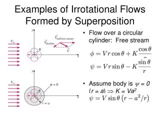
2. Examples of Irrotational Flows Formed by Superposition • Velocity field can be found by differentiating streamfunction • On the cylinder surface (r=a) Normal velocity (Ur) is zero, Tangential velocity (U) is non-zero slip condition.

3. Examples of Irrotational Flows Formed by Superposition • Compute pressure using Bernoulli equation and velocity on cylinder surface Turbulentseparation Laminarseparation Irrotational flow

4. Examples of Irrotational Flows Formed by Superposition • Integration of surface pressure (which is symmetric in x), reveals that the DRAG is ZERO. This is known as D’Alembert’s Paradox • For the irrotational flow approximation, the drag force on any non-lifting body of any shape immersed in a uniform stream is ZERO • Why? • Viscous effects have been neglected. Viscosity and the no-slip condition are responsible for • Flow separation (which contributes to pressure drag) • Wall-shear stress (which contributes to friction drag)

5. Boundary Layer (BL) Approximation • BL approximation bridges the gap between the Euler and NS equations, and between the slip and no-slip BC at the wall. • Prandtl (1904) introduced the BL approximation

6. Boundary Layer (BL) Approximation Not to scale To scale

7. Boundary Layer (BL) Approximation • BL Equations: we restrict attention to steady, 2D, laminar flow (although method is fully applicable to unsteady, 3D, turbulent flow) • BL coordinate system • x : tangential direction • y : normal direction

8. Boundary Layer (BL) Approximation • To derive the equations, start with the steady nondimensional NS equations • Recall definitions • Since , Eu ~ 1 • Re >> 1, Should we neglect viscous terms? No!, because we would end up with the Euler equation along with deficiencies already discussed. • Can we neglect some of the viscous terms?

9. Boundary Layer (BL) Approximation • To answer question, we need to redo the nondimensionalization • Use L as length scale in streamwise direction and for derivatives of velocity and pressure with respect to x. • Use  (boundary layer thickness) for distances and derivatives in y. • Use local outer (or edge) velocity Ue.

10. Boundary Layer (BL) Approximation • Orders of Magnitude (OM) • What about V? Use continuity • Since

11. Boundary Layer (BL) Approximation • Now, define new nondimensional variables • All are order unity, therefore normalized • Apply to x- and y-components of NSE • Details of derivation in textbook

12. Boundary Layer (BL) Approximation • Incompressible Laminar Boundary Layer Equations Continuity X-Momentum Y-Momentum

13. Boundary Layer Procedure • Solve for outer flow, ignoring the BL. Use potential flow (irrotational approximation) or Euler equation • Assume /L << 1 (thin BL) • Solve BLE • y = 0  no-slip, u=0, v=0 • y =  U = Ue(x) • x = x0  u = u(x0), v=v(x0) • Calculate , , *, w, Drag • Verify /L << 1 • If /L is not << 1, use * as body and goto step 1 and repeat

14. Boundary Layer Procedure • Possible Limitations • Re is not large enough  BL may be too thick for thin BL assumption. • p/y 0 due to wall curvature  ~ R • Re too large  turbulent flow at Re = 1x105. BL approximation still valid, but new terms required. • Flow separation

15. Boundary Layer Procedure • Before defining and * and are there analytical solutions to the BL equations? • Unfortunately, NO • Blasius Similarity Solutionboundary layer on a flat plate, constant edge velocity, zero external pressure gradient

16. Blasius Similarity Solution • Blasius introduced similarity variables • This reduces the BLE to • This ODE can be solved using Runge-Kutta technique • Result is a BL profile which holds at every station along the flat plate

17. Blasius Similarity Solution

18. Blasius Similarity Solution • Boundary layer thickness can be computed by assuming that  corresponds to point where U/Ue = 0.990. At this point,  = 4.91, therefore • Wall shear stress w and friction coefficient Cf,x can be directly related to Blasius solution Recall

19. Displacement Thickness • Displacement thickness * is the imaginary increase in thickness of the wall (or body), as seen by the outer flow, and is due to the effect of a growing BL. • Expression for * is based upon control volume analysis of conservation of mass • Blasius profile for laminar BL can be integrated to give (1/3 of )

20. Momentum Thickness • Momentum thickness  is another measure of boundary layer thickness. • Defined as the loss of momentum flux per unit width divided by U2 due to the presence of the growing BL. • Derived using CV analysis.  for Blasius solution, identical to Cf,x

21. Turbulent Boundary Layer Black lines: instantaneous Pink line: time-averaged Illustration of unsteadiness of a turbulent BL Comparison of laminar and turbulent BL profiles

22. Turbulent Boundary Layer • All BL variables [U(y), , *, ] are determined empirically. • One common empirical approximation for the time-averaged velocity profile is the one-seventh-power law

23. Turbulent Boundary Layer

24. Turbulent Boundary Layer • Flat plate zero-pressure-gradient TBL can be plotted in a universal form if a new velocity scale, called the friction velocity U, is used. Sometimes referred to as the “Law of the Wall” Velocity Profile in Wall Coordinates

25. Turbulent Boundary Layer • Despite it’s simplicity, the Law of the Wall is the basis for many CFD turbulence models. • Spalding (1961) developed a formula which is valid over most of the boundary layer • , B are constants

26. Pressure Gradients • Shape of the BL is strongly influenced by external pressure gradient (a) favorable (dP/dx < 0) (b) zero (c) mild adverse (dP/dx > 0) (d) critical adverse (w = 0) (e) large adverse with reverse (or separated) flow

27. Pressure Gradients • The BL approximation is not valid downstream of a separation point because of reverse flow in the separation bubble. • Turbulent BL is more resistant to flow separation than laminar BL exposed to the same adverse pressure gradient Laminar flow separates at corner Turbulent flow does not separate