Download
1 / 14
140 likes | 267 Views
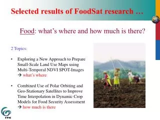
Selected results of FoodSat research … Food : what’s where and how much is there? 2 Topics: Exploring a New Approach to Prepare Small-Scale Land Use Maps using Multi-Temporal NDVI SPOT-Images what’s where

E N D
Selected results of FoodSat research … • Food: what’s where and how much is there? • 2 Topics: • Exploring a New Approach to Prepare Small-Scale Land Use Maps using Multi-Temporal NDVI SPOT-Images what’s where • Combined Use of Polar Orbiting and Geo-Stationary Satellitesto Improve Time Interpolation in Dynamic Crop Modelsfor Food Security Assessment how much is there
What’s where … by compiling existing data!! Used for mapping (Nizamabad, India): Time series of 147 SPOT-4 Vegetation decadal NDVI images (declouded) at 1-km2 resolution. Strong emphasis on temporal aspects reflecting vegetation phenology and practiced crop calendars.
Result-1: Unsupervised classification (ISODATA clustering) followed bysupervised grouping (based on profile behaviour) Output: a 1-km2 NDVI unit map with 11 NDVI-profiles as preliminary legend.
crossing Result-2: Using an existing (old) land cover map to define what each NDVI-unit represents. Output: Distinct sets of cover complexes by NDVI-unit.
Result-3: Using agricultural statistics by admin.area to define crops grown by NDVI-unit (through multiple regression). Output: Data of fraction by NDVI-unit and season, planted to specific crops.
Result-4: Combining results 1,2,3 and literature on crop calendars practiced, to prepare the final legend = final output. Section of the full legend ….
175 125 75 Jul Jul Jul Jul Jan Jan Jan Jan Sep Sep Sep Sep Mar Mar Mar Nov Nov Nov Nov May May May May Extra result: Monitoring land use modifications of irrigated areas, where during winter, rice is the dominant crop. 849 1038 961 P (apr-dec): 952 500 400 300 Rainfall (mm/month) NDVI 200 18 17 100 13,15 2002 2001 2000 1999 0 Mar May The NDVI-curves mostly reflect changes in areas cropped by year; changes could not be related directly to rainfall, but …by lack of power to run pumps!!
Key findings: • existing available data are combined to delineate / describe ‘what is where’ through data mining, • the generated map has 1 km2 pixels, and consists of ‘mixels’ representingunique land cover and land use complexes, • · map units are defined on the basis of their behaviour in time that tallies with signals provided by instruments used for monitoring, • · the map does not have a ‘salt-and-pepper’ appearance, but has clear delineable map units, while the method used was not sensitive to the size of identified units, • the supervised grouping following the unsupervised classification, yielded very good results regarding the generaliza-tion and stratification of the large spatial data set, • no specific field verification was required,though local expert knowledge of the authorsmatched the results.
How much is there…by spatial modelling!! • Defined by a production function as included in a crop growth model: • P,Y = f (light, temperature, C3/C4, canopyheating) gains losses
ΔT < 0 ΔT > 0 Canopy heating: a proxy for crop stress • Plant temperatures increase following reduced transpiration rates, caused by: • deficit of water (water stress), • reduction of biomass (by diseases or pestes), • high salinity in the soil water, • nutrient deficiencies and toxicities, • etc. • Plant temperatures can be estimated through Thermal Infrared Satellite Imagery.
Result-1: Combining TI-images of both polar orbiting and geo-stationary satellites and a crop growth model. Output: Software that pre-processes images of various sources and use them as input in a ‘spatial’ crop growth model (PSn).
Result-2: Cross-calibration of multi-sensor data. Output: Procedures that carry out sensor, time and place specific atmospheric and radiometric correction to generate sensor a-specific temperature measurements (split-window algorithm).
Result-3: duration/severity of crop stress detected using a temperature-based remotely sensed index (cfH2O; China) A(bove): NOAA data alone B(elow): NOAA/GMS-5 combined Duration first stress period: 1a: 2 days 1b: 6 days. Dry matter growth curves simulated with the PS-n model on the basis of canopy-ambient air temperature differences.
Key findings: • the method greatly reduces the computational data needs of crop growth models, • the method allows estimation of not just the H2O-limited production, but of “actual farmer’s production”, • drawbacks of polar-orbiters (rough temporal resolution) and geo-stationary satellites (poor radiometric signal) are eliminated by combining the two, • multi-sensor data can only be combined when cross-calibrated, • uncertainties in modeled losses are less when combining data from various RS-platforms.