Managing Flow Variability Process Capability
Managing Flow Variability Process Capability. These sides and note were prepared using Managing Business Flow processes. Anupindi , Chopra, Deshmukh , Van Mieghem , and Zemel.Pearson Prentice Hall.

Managing Flow Variability Process Capability
E N D
Presentation Transcript
Managing Flow VariabilityProcess Capability These sides and note were prepared using Managing Business Flow processes. Anupindi, Chopra, Deshmukh, Van Mieghem, and Zemel.Pearson Prentice Hall. Few of the graphs of the slides of Prentice Hall for this book, originally prepared by professor Deshmukh. A Statement for Quality Goes Here
Fraction of Output within Specifications The fraction of the process output that meets customer specifications. We can compute this fraction by: the histogram of the actual observation, or using Normal distribution. Ex. 9.7: US: 85kg; LS: 75 kg (the range of performance variation that customer is willing to accept). Histogram: In an observation of 100 samples, the process is 74% capable of meeting customer requirements, and 26% defectives!!! Assume door weight, W, follows Normal random variable with mean = 82.5 kg and standard deviation at 4.2 kg, Prob(75 ≤ W ≤ 85) = Prob (W ≤ 85) - Prob (W ≤ 75) = Prob ((75-82.5)/4.2 ≤ z ≤ (85-82.5)/4.2 ) = Prob(Z≤.5952) = .724, Prob(Z ≤ -1.79) = .0367 Prob (75 ≤ W ≤ 85) = 0.724 - 0.0367 = .6873
9.4.1 Fraction of Output within Specifications SO with normal approximation, the process is capable of producing 69% of doors within the specifications, or delivering 31% defective doors!!! Specifications refer to individualdoors, not AVERAGES. We cannot comfort customer that there is a 30% chance that they’ll get doors that is either too light or too heavy!!!
Process Capability Ratios (Cpkand Cp) • Process capability ratio, Cpk, his measure is based on the observation that for a normal distribution, if the mean is 3 standard deviations above the lower specification LS (or below the upper specification US), there is very little chance of a product characteristic falling below LS (or above US). • Compute (US –)/3and ( – LS)/3 • The higher these values, the more capable the process is in meeting specifications. • Cpk =min [(US –)/3, ( – LS)/3]
9.4.2 Process Capability Ratios (C pk and Cp) • Cpk of 1+- represents a capable process • Not too high (or too low) • Lower values = only better than expected quality Ex: processing cost, delivery time delay, or # of error per transaction process • If the process is properly centered • Cpk is then either: (US- μ)/3σ or (μ -LS)/3σ As both are equal for a centered process.
9.4.2 Process Capability Ratios (C pk and Cp) cont… • Therefore, for a correctly centered process, we may simply define the process capability ratio as: • Cp = (US-LS)/6σ (.3968, as calculated later) Numerator = voice of the customer / denominator = the voice of the process • Recall: with normal distribution: Most process output is 99.73% falls within +-3σ from the μ. • Consequently, 6σ is sometimes referred to as the natural tolerance of the process. Ex: 9.8 Cpk = min[(US- μ)/3σ , (μ -LS)/3σ ] = min {(85-82.5)/(3)(4.2)], (82.5-75)/(3)(4.2)]} = min {.1984, .5952} =.1984
9.4.2 Process Capability Ratios (C pk and Cp) • If the process is correctly centered at μ = 80kg (between 75 and 85kg), we compute the process capability ratio as Cp = (US-LS)/6σ = (85-75)/[(6)(4.2)] = .3968 • NOTE: Cpk = .1984 (or Cp = .3968) does not mean that the process is capable of meeting customer requirements by 19.84% (or 39.68%), of the time. It’s about 69%. • Defects are counted in parts per million (ppm) or ppb, and the process is assumed to be properly centered. IN THIS CASE, If we like no more than 100 defects per million (.01% defectives), we SHOULD HAVE the probability distribution of door weighs so closely concentrated around the mean that the standard deviation is 1.282 kg, or Cp=1.3 (see Table 9.4) Test: σ = (85-75)/(6)(1.282)] = 1.300kg
9.4.3 Six-Sigma Capability • The 3rd process capability • Known as Sigma measure, which is computed as • S = min[(US- μ /σ), (μ -LS)/σ] (= min(.5152,1.7857) = .5152 to be calculated later) • S-Sigma process If process is correctly centered at the middle of the specifications, S = [(US-LS)/2σ] Ex: 9.9 Currently the sigma capability of door making process is S=min(85-82.5)/[(2)(4.2)] = .5952 By centering the process correctly, its sigma capability increases to S=min(85-75)/[(2)(4.2)] = 1.19 THUS, with a 3σ that is correctly centered, the US and LS are 3σ away from the mean, which corresponds to Cp=1, and 99.73% of the output will meet the specifications.
9.4.3 Six-Sigma Capability cont… • SIMILARLY, a correctly centered six-sigma process has a standard deviation so small that the US and LS limits are 6σ from the mean each. • Extraordinary high degree of precision. Corresponds to Cp=2 or 2 defective units per billion produced!!! (see Table 9.5) • In order for door making process to be a six-sigma process, its standard deviation must be: σ = (85-75)/(2)(6)] = .833kg • Adjusting for Mean Shifts Allowing for a shift in the mean of +-1.5 standard deviation from the center of specifications. Allowing for this shift, a six-sigma process amounts to producing an average of 3.4 defective units per million. (see table 9.5)
9.4.3 Six-Sigma Capability cont… • Why Six-Sigma? • See table 9.5 • Improvement in process capabilities from a 3-sigma to 4-sigma = 10-fold reduction in the fraction defective (66810 to 6210 defects) • While 4-sigma to 5-sigma = 30-fold improvement (6210 to 232 defects) • While 5-sigma to 6-sigma = 70-fold improvement (232 to 3.4 defects, per million!!!). • Average companies deliver about 4-sigma quality, where best-in-class companies aim for six-sigma.
9.4.3 Six-Sigma Capability cont… • Why High Standards? • The overall quality of the entire product/process that requires ALL of them to work satisfactorily will be significantly lower. Ex: If product contains 100 parts and each part is 99% reliable, the chance that the product (all its parts) will work is only (.99)100 = .366, or 36.6%!!! • Also, costs associated with each defects may be high • Expectations keep rising
9.4.3 Six-Sigma Capability cont… • Safety capability - We may also express process capabilities in terms of the desired margin [(US-LS)-zσ] as safety capability - It represents an allowance planned for variability in supply and/or demand - Greater process capability means less variability - If process output is closely clustered around its mean, most of the output will fall within the specifications - Higher capability thus means less chance of producing defectives - Higher capability = robustness
9.4.4 Capability and Control • So in Ex. 9.7: the production process is not performing well in terms of MEETING THE CUSTOMER SPECIFICATIONS. Only 69% meets output specifications!!! (See 9.4.1: Fraction of Output within Specifications) • Yet in example 9.6, “the process was in control!!!”, or WITHIN US & LS LIMITS. • Meeting customer specifics: indicates internal stability and statistical predictability of the process performance. • In control (aka within LS and US range): ability to meet external customer’s requirements. • Observation of a process in control ensures that the resulting estimates of the process mean and standard deviation are reliable so that our measurement of the process capability is accurate.
9.5 Process Capability Improvement • Shift the process mean • Reduce the variability • Both
9.5.1 Mean Shift • Examine where the current process mean lies in comparison to the specification range (i.e. closer to the LS or the US) • Alter the process to bring the process mean to the center of the specification range in order to increase the proportion of outputs that fall within specification
Ex 9.10 • MBPF garage doors (currently) -specification range: 75 to 85 kgs -process mean: 82.5 kgs -proportion of output falling within specifications: .6873 • The process mean of 82.5 kgs was very close to the US of 85 kgs (i.e. too thick/heavy) • To lower the process mean towards the center of the specification range the supplier could change the thickness setting on their rolling machine
Ex 9.10 Continued • Center of the specification range: (75 + 85)/2 = 80 kgs • New process mean: 80 kgs • If the door weight (W) is a normal random variable, then the proportion of doors falling within specifications is: Prob (75 =< W =< 85) • Prob (W =< 85) – Prob (W =< 75) • Z = (weight – process mean)/standard deviation • Z = (85 – 80)/4.2 = 1.19 • Z = (75 – 80)/4.2 = -1.19
Ex 9.10 Continued • [from table A2.1 on page 319] Z = 1.19 .8830 Z = -1.19 (1 - .8830) .1170 • Prob (W =< 85) – Prob (W =< 75) = .8830 - .1170 = .7660 • By shifting the process mean from 82.5 kgs to 80 kgs, the proportion of garage doors that falls within specifications increases from .6873 to .7660
9.5.2 Variability Reduction • Measured by standard deviation • A higher standard deviation value means higher variability amongst outputs • Lowering the standard deviation value would ultimately lead to a greater proportion of output that falls within the specification range
9.5.2 Variability Reduction Continued • Possible causes for the variability MBPF experienced are: -old equipment -poorly maintained equipment -improperly trained employees • Investments to correct these problems would decrease variability however doing so is usually time consuming and requires a lot of effort
Ex 9.11 • Assume investments are made to decrease the standard deviation from 4.2 to 2.5 kgs • The proportion of doors falling within specifications: Prob (75 =< W =< 85) • Prob (W =< 85) – Prob (W =< 75) • Z = (weight – process mean)/standard deviation • Z = (85 – 80)/2.5 = 2.0 • Z = (75 – 80)/2.5 = -2.0
Ex 9.11 Continued • [from table A2.1 on page 319] Z = 2.0 .9772 Z = -2.0 (1 - .9772) .0228 • Prob (W =< 85) – Prob (W =< 75) = .9772 - .0228 = .9544 • By shifting the standard deviation from 4.2 kgs to 2.5 kgs and the process mean from 82.5 kgs to 80 kgs, the proportion of garage doors that falls within specifications increases from .6873 to .9544
9.5.3 Effect of Process Improvement on Process Control • Changing the process mean or variability requires re-calculating the control limits • This is required because changing the process mean or variability will also change what is considered abnormal variability and when to look for an assignable cause
9.6 Product and Process Design • Reducing the variability from product and process design -simplification -standardization -mistake proofing
Simplification • Reduce the number of parts (or stages) in a product (or process) -less chance of confusion and error • Use interchangeable parts and a modular design -simplifies materials handling and inventory control • Eliminate non-value adding steps -reduces the opportunity for making mistakes
Standardization • Use standard parts and procedures -reduces operator discretion, ambiguity, and opportunity for making mistakes
Mistake Proofing • Designing a product/process to eliminate the chance of human error -ex. color coding parts to make assembly easier -ex. designing parts that need to be connected with perfect symmetry or with obvious asymmetry to prevent assembly errors
9.6.2 Robust Design • Designing the product in a way so its actual performance will not be affected by variability in the production process or the customer’s operating environment • The designer must identify a combination of design parameters that protect the product from the process related and environment related factors that determine product performance
QUESTIONS ???