Download

1 / 60
600 likes | 727 Views
This paper discusses the optimization of sensor placement for monitoring water quality, focusing on the detection of algal blooms that threaten freshwater supplies for millions. With the potential to impact over 4 million people and cost billions in cleanup, the need for effective monitoring strategies is critical. Leveraging probabilistic models and algorithms, this work aims to enhance our capability to sense large spatial phenomena in lakes and rivers, ensuring timely responses to water contamination and promoting better water management practices.

E N D
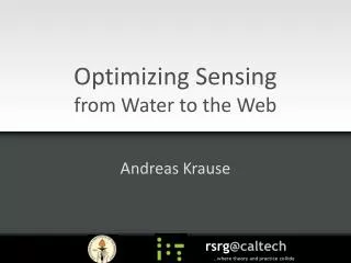
Optimizing Sensingfrom Water to the Web Andreas Krause rsrg@caltech ..where theory and practice collide TexPoint fonts used in EMF. Read the TexPoint manual before you delete this box.: AAAAAAAAAAA
Monitoring algal blooms Algal blooms threaten freshwater 4 million people without water 1300 factories shut down $14.5 billion to clean up Other occurrences in Australia, Japan, Canada, Brazil, Mexico, Great Britain, Portugal, Germany … Growth processes still unclear Need to characterize growth in the lakes, not in the lab! Tai Lake China 10/07 MSNBC
Depth Predict atunobservedlocations Location across lake Monitoring rivers and lakes[IJCAI ‘07] • Need to monitor large spatial phenomena • Temperature, nutrient distribution, fluorescence, … NIMSKaiseret.al.(UCLA) Can only make a limited number of measurements! Color indicates actual temperature Predicted temperature Use robotic sensors tocover large areas Where should we sense to get most accurate predictions?
Hach Sensor Monitoring water networks[J Wat Res Mgt 2008] • Contamination of drinking watercould affect millions of people Contamination Sensors Simulator from EPA ~$14K Place sensors to detect contaminations “Battle of the Water Sensor Networks” competition Where should we place sensors to quickly detect contamination?
Sensing problems • Want to learn something about the state of the world • Estimate water quality in a geographic region, detect outbreaks, … • We can choose (partial) observations… • Make measurements, place sensors, choose experimental parameters … • … but they are expensive / limited • hardware cost, power consumption, grad student time … Want to cost-effectively get most useful information! Fundamental problem in Machine Learning:How do we decide what to learn from?
Related work Sensing problems considered in Experimental design (Lindley ’56, Robbins ’52…), Spatial statistics (Cressie ’91, …), Machine Learning (MacKay ’92, …), Robotics (Sim&Roy ’05, …), Sensor Networks (Zhao et al ’04, …), Operations Research (Nemhauser ’78, …) Existing algorithms typically • Heuristics: No guarantees! Can do arbitrarily badly. • Find optimal solutions (Mixed integer programming, POMDPs): Very difficult to scale to bigger problems.
Contributions Theoretical: Approximation algorithms that have theoretical guarantees and scale to large problems Applied: Empirical studies with real deployments and large datasets
Model-based sensing • Utility of placing sensors based on model of the world • For lake monitoring: Learn probabilistic models from data (later) • For water networks: Water flow simulator from EPA • For each subset A µ V compute “sensing quality” F(A) Model predicts High impact Lowimpactlocation Contamination Medium impactlocation S3 S1 S2 S3 S4 S2 Sensor reducesimpact throughearly detection! S1 S4 Set V of all network junctions S1 Low sensing quality F(A)=0.01 High sensing quality F(A) = 0.9
Sensing locations Sensing quality Sensing cost Sensing budget Optimizing sensing / Outline Sensor placement Robust sensing Complex constraints Sequential sensing
Sensor placement Given: finite set V of locations, sensing quality F Want: A*µ V such that Typically NP-hard! How well can this simple heuristic do? S3 S1 S5 S2 S4 Greedy algorithm: Start with A = ; For i = 1 to k s* := argmaxs F(A [ {s}) A := A [ {s*} S6
Performance of greedy algorithm Greedy score empirically close to optimal. Why? Optimal Greedy Population protected (higher is better) Small subset of Water networks data Number of sensors placed
Key property: Diminishing returns Placement A = {S1, S2} Placement B = {S1, S2, S3, S4} S2 S2 S3 S1 S1 S4 Theorem [Krause et al., J Wat Res Mgt ’08]: Sensing quality F(A) in water networks is submodular! Adding S’ will help a lot! Adding S’ doesn’t help much S’ New sensor S’ + S’ B Large improvement Submodularity: A + S’ Small improvement For Aµ B, F(A [ {S’}) – F(A) ¸ F(B [ {S’}) – F(B)
~63% One reason submodularity is useful Theorem [Nemhauser et al ‘78] Greedy algorithm gives constant factor approximation F(Agreedy) ¸ (1-1/e) F(Aopt) • Greedy algorithm gives near-optimal solution! • Guarantees best possible unless P = NP! Many more reasons, sit back and relax…
Leanforward Leanleft Slouch Building a Sensing Chair [UIST ‘07] • People sit a lot • Activity recognition inassistive technologies • Seating pressure as user interface Equipped with 1 sensor per cm2! Costs $16,000! Can we get similar accuracy with fewer, cheaper sensors? 82% accuracy on 10 postures! [Tan et al]
How to place sensors on a chair? • Sensor readings at locations V as random variables • Predict posture Y using probabilistic model P(Y,V) • Pick sensor locations A* µ V to minimize entropy: Possible locations V Placed sensors, did a user study: Theorem: Information gain is submodular!*[UAI’05] Similar accuracy at <1% of the cost! *See store for details
Battle of the Water Sensor Networks Competition • Real metropolitan area network (12,527 nodes) • Water flow simulator provided by EPA • 3.6 million contamination events • Multiple objectives: Detection time, affected population, … • Place sensors that detect well “on average”
30 25 E H G 20 G E H 15 Total ScoreHigher is better G 10 G D H D G 5 0 Gueli Trachtman Guan et. al. Berry et. al. Dorini et. al. Wu & Walski Huang et. al. Preis & Ostfeld Propato & Piller Our approach Ghimire & Barkdoll Ostfeld & Salomons Eliades & Polycarpou BWSN Competition results [Ostfeld et al., J Wat Res Mgt 2008] • 13 participants • Performance measured in 30 different criteria G: Genetic algorithm D: Domain knowledge E: “Exact” method (MIP) H: Other heuristic 24% better performance than runner-up!
300 Exhaustive search (All subsets) 200 Naive Running time (minutes) greedy ubmodularity to the rescue: 100 Fast greedy 0 1 2 3 4 5 6 7 8 9 10 Number of sensors selected What was the trick? , 16 GB in main memory (compressed) Advantage through theory and engineering! Simulated all on 2 weeks / 40 processors 152 GB data on disk Very accurate sensing quality 3.6M contaminations Very slow evaluation of F(A) 30 hours/20 sensors 6 weeks for all30 settings Lower is better Using “lazy evaluations”:1 hour/20 sensors Done after 2 days!
S3 S2 S4 S1 What about worst-case? Knowing the sensor locations, an adversary contaminates here! S3 S2 S4 S1 Placement detects well on “average-case” (accidental) contamination Very different average-case impact,Same worst-case impact Where should we place sensors to quickly detect in the worst case?
Optimizing for the worst case • Separate utility function Fi with each contamination i • Fi(A) = impact reduction by sensors A for contamination i Want to solve Each of the Fi is submodular Unfortunately, mini Fi not submodular! How can we solve this robust sensing problem? Contamination at node s Sensors A Fs(C) is high Fs(B) is low Fs(A) is high Sensors C Sensors B Contamination at node r Fr(A) is low Fr(B) is high Fr(C) is high
Outline Sensor placement Robust sensing Complex constraints Sequential sensing
How does the greedy algorithm do? V={ , , } Greedy does arbitrarily badly. Is there something better? Can only buy k=2 Greedy picks first Hence we can’t find any approximation algorithm. Optimalsolution Then, canchoose only or Optimal score: 1 Or can we? Greedy score: Theorem [NIPS ’07]: The problem max|A|· k mini Fi(A) does not admit any approximation unless P=NP
Alternative formulation If somebody told us the optimal value, can we recover the optimal solution A*? Need to find Is this any easier? Yes, if we relax the constraint |A| · k
c Problem 1 (last slide) Problem 2 Solving the alternative problem Trick: For each Fi and c, define truncation Fi(A) F’i,c(A) |A| Same optimal solutions!Solving one solves the other Non-submodular Don’t know how to solve Submodular!Can use greedy!
Back to our example • Guess c=1 • First pick • Then pick Optimal solution! How do we find c? Do binary search!
Truncationthreshold(color) Saturate Algorithm [NIPS ‘07] • Given: set V, integer k and submodular functions F1,…,Fm • Initialize cmin=0, cmax = mini Fi(V) • Do binary search: c = (cmin+cmax)/2 • Greedily find AG such that F’avg,c(AG) = c • If |AG| · k: increase cmin • If |AG| > k: decrease cmax until convergence
Theoretical guarantees Theorem:If there were a polytime algorithm with better factor < , then NP µ DTIME(nlog log n) Theorem: The problem max|A|· k mini Fi(A) does not admit any approximation unless P=NP Theorem: Saturate finds a solution AS such that mini Fi(AS) ¸ OPTk and |AS| · k where OPTk = max|A|·k mini Fi(A) = 1 + log maxsi Fi({s})
(often) submodular [Das & Kempe ’08] Example: Lake monitoring • Monitor pH values using robotic sensor transect Prediction at unobservedlocations Observations A True (hidden) pH values pH value Var(s | A) Use probabilistic model(Gaussian processes)to estimate prediction error Position s along transect Where should we sense to minimize our maximum error? Robust sensing problem!
2.5 Greedy 2 Maximum marginal variance 1.5 Simulated Annealing 1 Saturate 0.5 0 20 40 60 80 100 Number of sensors Comparison with state of the art Algorithm used in geostatistics: Simulated Annealing [Sacks & Schiller ’88, van Groeningen & Stein ’98, Wiens ’05,…] 7 parameters that need to be fine-tuned better Saturate is competitive & 10x faster No parameters to tune! Precipitation data Environmental monitoring
Greedy Simulated Annealing Saturate Results on water networks 60% lower worst-case detection time! 3000 No decreaseuntil allcontaminationsdetected! 2500 2000 Maximum detection time (minutes) 1500 Lower is better 1000 500 Water networks 0 0 10 20 Number of sensors
Outline Sensor placement Robust sensing Complex constraints Sequential sensing
Other aspects: Complex constraints maxA F(A) or maxA mini Fi(A) subject to • So far: |A| · k • In practice, more complex constraints: Sensors need to communicate (form a routing tree) Locations need to be connected by paths[IJCAI ’07, AAAI ’07] Lake monitoring Building monitoring
1 2 2 1.5 relay node 1 1 1 1 2 No communicationpossible! C(A) = 1 relay node C(A) = 3.5 F(A) = 3.5 2 2 Naïve approach: Greedy-connect • Simple heuristic: Greedily optimize sensing quality F(A) • Then add nodes to minimize communication cost C(A) 2 2 relay node F(A) = 0.2 Most informative F(A) = 4 F(A) = 4 C(A) = 3 C(A) = 10 C(A) = 10 2 Secondmost informative relay node 2 2 efficientcommunication! Not veryinformative Very informative, High communicationcost! Communication cost = Expected # of trials (learned using Gaussian Processes) Want to find optimal tradeoff between information and communication cost
The pSPIEL Algorithm[IPSN ’06 – Best Paper Award] pSPIEL: padded Sensor Placements at Informative and cost-Effective Locations Theorem: pSPIEL finds a placement A with sensing quality F(A)¸(1) OPTFcommunication cost C(A)·O(log |V|) OPTC Real deployment at CMUArchitecture department 44% lower error and 19% lower communication costthan placement by domain expert!
Outline Sensor placement Robust sensing Complex constraints Sequential sensing
Other aspects: Sequential sensing • You walk up to a lake, but don’t have a model • Want sensing locations to learn the model (explore) and predict well (exploit) • Chosen locations depend on measurements! [ICML ’07] Exploration—Exploitation analysis for Active Learning in Gaussian Processes
Summary so far All these applications involve physical sensing. Now for something completely different.Let’s jump from water… Submodularity in sensing optimizationGreedy is near-optimal [UAI ’05, JMLR ’07, KDD ’07] Path planning Communication constraints Constrained submodular optimization pSPIEL gives strong guarantees[IJCAI ’07, IPSN ’06, AAAI ‘07] Robust sensing Greedy fails badly Saturate is near-optimal[NIPS ’07] Sequential sensing Exploration Exploitation Analysis [ICML ’07, IJCAI ‘05]
… to the Web! You have 10 minutes each day for reading blogs / news. Which of the million blogs should you read?
Cascades in the Blogosphere[KDD 07 – Best Paper Award] Learn aboutstory after us! Time Information cascade Which blogs should we read to learn about big cascades early?
Water vs. Web • In both problems we are given • Graph with nodes (junctions / blogs) and edges (pipes / links) • Cascades spreading dynamically over the graph (contamination / citations) • Want to pick nodes to detect big cascades early Placing sensors inwater networks Selectinginformative blogs vs. In both applications, utility functions submodular [Generalizes Kempe et al, KDD ’03]
400 0.7 Greedy Exhaustive search 0.6 (All subsets) 300 0.5 Lower is better Naive 0.4 Higher is better Running time (seconds) Cascades captured 200 greedy In-links 0.3 All outlinks 100 0.2 # Posts Fast greedy Random 0.1 0 0 1 2 3 4 5 6 7 8 9 10 0 20 40 60 80 100 Number of blogs selected Number of blogs Blog selection Performance on Blog selection Outperforms state-of-the-art heuristics 700x speedup using submodularity! Blog selection ~45k blogs
Cascades captured Number of posts (time) allowed Taking “attention” into account • Naïve approach: Just pick 10 best blogs • Selects big, well known blogs (Instapundit, etc.) • These contain many posts, take long to read! Cost/benefitanalysis Ignoring cost x 104 Cost-benefit optimization picks summarizer blogs!
Greedy on future 0.25 Test on future “Cheating” 0.2 Greedy on historic Test on future 0.15 Cascades captured 0.1 Detect poorlyhere! Detect wellhere! 0.05 0 0 1000 2000 3000 4000 Number of posts (time) allowed Predicting the “hot” blogs • Want blogs that will be informative in the future • Split data set; train on historic, test on future Detects on training set Blog selection “overfits”to training data! Poor generalization!Why’s that? Want blogs thatcontinue to do well! Let’s see whatgoes wrong here.
F5 (A)=.02 F4(A)=.01 F3 (A)=.6 F2 (A)=.8 F1(A)=.5 Robust optimization “Overfit” blog selection A Fi(A) = detections in interval i Optimizeworst-case Detections using Saturate “Robust” blog selection A* Robust optimization Regularization!
Robust solution Test on future Greedy on future 0.25 Test on future “Cheating” 0.2 Greedy on historic Test on future 0.15 Sensing quality 0.1 0.05 0 0 1000 2000 3000 4000 Number of posts (time) allowed Predicting the “hot” blogs 50% better generalization!
Submodularity in sensing optimizationGreedy is near-optimal [UAI ’05, JMLR ’07, KDD ’07] Path planning Communication constraints Constrained submodular optimization pSPIEL gives strong guarantees[IJCAI ’07, IPSN ’06] Robust sensing Greedy fails badly Saturate is near-optimal[NIPS ’07] Sequential sensing Exploration Exploitation Analysis [ICML ’07] Future work Robust optimization better generalization Constrained optimization better use of “attention” Thesis in a box
Sensys ‘05 ICML ‘06 ISWC ‘06 Trans MobComp ‘06 UAI ‘05 Future work Algorithmic and statistical machine learning Fundamental questions in Information Acquisition and Interpretation Machine learningand sensing in natural sciencesand engineering Machine learning and optimizationon the web Thesis in a box
Structure in ML / AI problems • Structural insights help us solve challenging problems • Shameless plug: Tutorial at ICML 2008 ML “next 10 years:” Submodularity New structural properties ML last 10 years: Convexity Kernel machines SVMs, GPs, MLE…
Future work Algorithmic and statistical machine learning Fundamental questions in Information Acquisition and Interpretation Machine learningand sensing in natural sciencesand engineering Machine learning and optimizationon the web Thesis in a box
Fundamental bottlenecks in information acquisition Attention extremely scarce,non-renewable! Web User Privacy • Preliminary results • Utility/Privacy in Personalized search. Submodularity is key! • Planned study: data from 2 million blogs from spinn3r.com