Download
1 / 29
330 likes | 425 Views
This text discusses groundwater permeability, ill-conditioned problems, and nonstationary spatial data analysis using Gaussian processes and wavelet basis. Learn how to solve forward and inverse groundwater flow problems with regularization techniques and statistical methods.

E N D
Groundwater permeability Easy to solve the forward problem: flow of groundwater given permeability of aquifer Inverse problem: determine permeability from flow (usually of tracers) With some models enough to look at first arrival of tracer at each well (breakthrough times)
Notation is permeability b is breakthrough times expected breakthrough times Illconditioned problems: different permeabilities can yield same flow Use regularization by prior on log() MRF Gaussian Convolution with MRF (discretized)
MRF prior where and nj=#{i:i~j}
Kim, Mallock & Holmes, JASA 2005 Analyzing Nonstationary Spatial Data UsingPiecewise Gaussian Processes Studying oil permeability Voronoi tesselation (choose M centers from a grid) Separate power exponential in each regions
Nott & Dunsmuir, 2002, Biometrika Consider a stationary process W(s), correlation R, observed at sites s1,..,sn. Write (s) has covariance function
More generally Consider k independent stationary spatial fields Wi(s) and a random vector Z. Write and create a nonstationary process by Its covariance (with =Cov(Z)) is
Fig. 2. Sydney wind pattern data. Contours of equal estimated correlation with two different fixed sites, shown by open squares: (a) location 33·85°S, 151·22°E, and (b) location 33·74°S, 149·88°E. The sites marked by dots show locations of the 45 monitored sites.
Karhunen-Loéve expansion There is a unique representation of stochastic processes with uncorrelated coefficients: where the k(s) solve and are orthogonal eigenfunctions. Example: temporal Brownian motion C(s,t)=min(s,t) k(s)=21/2sin((k-1/2)t)/((k-1/2)) Conversely,
Discrete case Eigenexpansion of covariance matrix Empirically SVD of sample covariance Example: squared exponential k=1 5 20
Tempering Stationary case: write with covariance To generalize this to a nonstationary case, use spatial powers of the k: Large corresponds to smoother field
Estimating (s) Regression spline Knots ui picked using clustering techniques Multivariate normal prior on the ’s.
Tempering More smoothness More fins structure
Covariances A B C D
Karhunen-Loeve expansionrevisited and where ai are iid N(0,i) Idea: use wavelet basis instead of eigenfunctions, allow for dependent ai
Spatial wavelet basis Separates out differences of averages at different scales Scaled and translated basic wavelet functions
Estimating nonstationary covariance using wavelets 2-dimensional wavelet basis obtained from two functions and: First generation scaled translates of all four; subsequent generations scaled translates of the detail functions. Subsequent generations on finer grids. detail functions
Covariance expansion For covariance matrix write Useful if D close to diagonal. Enforce by thresholding off-diagonal elements (set all zero on finest scales)
Surface ozone model ROM, daily average ozone 48 x 48 grid of 26 km x 26 km centered on Illinois and Ohio. 79 days summer 1987. 3x3 coarsest level (correlation length is about 300 km) Decimate leading 12 x 12 block of D by 90%, retain only diagonal elements for remaining levels.
Some open questions Multivariate Kronecker structure Nonstationarity Covariates causing nonstationarity (or deterministic models) Comparison of models of nonstationarity Mean structure