Download

1 / 45
660 likes | 2.74k Views
9. PERMEABILITY. Introduction. Behavior. Applications. Introduction. Soils are permeable due to the existence of interconnected voids. One of the most important consideration in soil mechanics is the effects of water in the soil on its engineering properties, and hence behavior.

E N D
Introduction Behavior Applications
Introduction • Soils are permeable due to the existence of interconnected voids. • One of the most important consideration in soil mechanics is the effects of water in the soil on its engineering properties, and hence behavior. • Most of geotechnical engineering problems somehow have water associated with them in various ways.
Permeability is one of the most important soil properties of interest to geotechnical engineering. • The following applications illustrate the importance of permeability in geotechnical design: • Permeability influences the rate of settlement of a saturated soil under load. • The design of earth dams is very much based upon the permeability of the soils used. Filters made of soils are designed based upon their permeability. • The stability of slopes and retaining walls can be greatly affected by the permeability of the soils • Permeability of soils is required in solving pumping seepage water from construction excavations.
Definition of Permeability • Permeability is a measure of a given porous medium ability to permit fluid flow through its voids. • Any material with voids is Porous and if the voids are interconnected, possesses permeability. • Therefore, rock, concrete, soil, and many engineering materials are both POROUS and PERMEABLE. However, among them soils, even in their densest state, are more permeable.
DARCY’S LAW FOR FLOW THROUGH POROUS MEDIA • Fluid flow can be described or classified in different ways like: • Steady vs. Unsteady • Laminar vs. Turbulent • 1-D vs. 3D • In our discussion in this chapter we will assume that the flow is laminar. This really is the case in most soils. • Whether the flow is steady or not and the number of dimensions we consider, this will be decided when we present SEEPAGE in the following chapter.
= loss of head between two points. • A French engineer named Darcy (1856) noticed that the velocity of the drainage drinking water flowing to a village named Dijon was • Proportional to the difference in elevation between the water’s entry point and its discharge point. • Inversely proportional to the distance over which the change in elevation occurred. Where: n = discharge velocity, which is the quantity of water flowing in unit time through a unit GROUS cross-sectional area of soil at rightangles to the direction of flows. L = Distance over which the change or loss of head occurs.
The ratio is termed the HYDRAULIC GRADIENT, and is denoted by the symbol i. Therefore, Eq. 1 becomes: • Darcy’ introduced a constant of proportionality called the Darcy Coefficient of Permeability, k and Eq. 2 becomes: • Commonly in civil engineering k is called simply hydraulic conductivity or the coefficient of permeability or, even more simply, the Permeability. • Eq. 3 is called Darcy’s law. It was primarily based on the observations made by Darcy for flow of water through clean sands.
Assumptions in Deriving Darcy’s Law I. Soils • Homogeneous & isotropic • Fully saturated II. Flow • The flow is laminar, no turbulent flows • The flow is in steady state, no temporal variation
Variation of Velocity with Hydraulic Gradient When the hydraulic gradient is increased gradually, the flow remains laminar in Zones I and II, and the velocity, v, bears a linear relationship to the hydraulic gradient. At a higher hydraulic gradient, the flow becomes turbulent (Zone III). When the hydraulic gradient is decreased, laminar flow conditions exist only in Zone I.
Variation of Velocity with Hydraulic Gradient At high gradient the flow will be turbulent and the relationship between v and I will not be linear. Hence Eq. 2 may not be valid. This is the case in gravels and very coarse sands. However, in most soil the flow of water through the voids can be considered LAMINAR and Eq. 2 is valid.
Is Darcy's law valid for very low hydraulic gradients? Proposition Darcy’s Law These equations imply that for very low hydraulic gradients, the relationship between v and i is nonlinear (only study by Hansbo, 1960) several other studies refute the preceding findings. Mitchell (1976) discussed these studies in detail. Taking all points into consideration, he concluded that Darcy’s law is valid. Conclusion: Darcy’s law is valid even for very low hydraulic gradients
FLOW RATE (Flux) • If A is the cross-sectional area through which flow is occurring, the flow rate, q, is determined by: or QUANTITY OF FLOW • If flow occurs over a period of time t, the total quantity of water Q flowing during this period can be found as: All terms in Eq. (5) are easily measured or determined except k. Next we will discuss techniques in evaluating k. But first we will address some important concepts regarding hydraulicgradient. or
To determine the quantity of flow, two parameters are needed * k = hydraulic conductivity (how permeable the soil medium) * i = hydraulic gradient (how large is the driving head) i can be determined • From the head loss and geometry….. (1-D case) • Flow net (nextchapter)……….(2D case) k can be determined using: • Laboratory Testing • Field Testing • Empirical Equations
Heads & Hydraulic Gradient Bernoulli’s Equation • According to Bernoulli's equation, the total energy available, described as a measurable distance (called head) above a reference datum is: (6)
In soils seepage velocity is normally very small (further if it is squared) that VELOCITY HEAD can be neglected. Therefore, the totalhead at any point is given as: (7) The pressure head at a point can be measured by inserting a PIEZOMETER TUBE into the pipe. The level will rise to a level representing the current pressure head at the that point. (If the flow is steady and the velocity head =0)
Piezometric Levels or Heads • The levels to which water rises in the piezometer tubes situated at points A and B are know as the piezometric levels of points A and B, respectively. • The loss of head between point A and B is given by: (8) • The hydraulic gradient (or head loss) is as defined before expressed as: (9) • It is the SLOPE of the ENERGY LINE defined by the free surface of flowing water in OPEN CHANNELS or the slope of the PIEZOMETRIC HEADS or LEVELS between two points in CONFINED FLOW.
Tricky case!! Remember always to look at total head uB/gw uA/gw
Remarks • A standpipe referred to as a PIEZOMETER is used for measuring pressure. It operates by converting pressurehead to the more readily measurable elevation head. • The quantity (hp+he) is called the piezometric head , piezometric level, or total head since it is the head that would be measured by a piezometer referenced to some datum plane. • The elevation of the water column in the standpipe is the TOTAL HEAD (hp +He), whereas the actual height of rise of the water column in the standpipe is the PRESSURE HEAD, hp. • Elevation head at a point = Extent of that point from the datum. • It is most often convenient to establish the datum plane at the tail water elevation.
Illustration of Heads Example 1 C hp(B) B hp(A) he(C) Total Head at A, B, C he(B) A he(A) Datum Remember always to look at total head
DISCHARGE AND SEEPAGE VELOCITIES • In Eq. (1), v is the discharge (apparent) seepage velocity of water based on the gross cross-sectional area of the soil, or (10) • However, water cannot be flowing through solid particles but only through the voids or pores between the grains. • The average velocity at which the water flows through the soil pores is obtained by: (11) vs is called the SEEPAGE VELOCITY
From the law of conservation of mass (for incompressive steady state flow, this low reduces to the EQUATION OF CONTINUITY), we get (or from Eqs. (10), (11): Therefore But with the 3rd dimension Hence (12)
Remarks • Eq. (12) indicates the relationship between the discharge velocity and the seepage velocity. • Since 0%< n < 100%, it follows that seepage velocity is always greater than the discharge (superficial) velocity. • n is also called the apparent seepage velocity. It is a superficial, fiction but convenient engineering velocity. (Also called velocity of approach). • ns > n not only because Av<A but also because the flow is not straight –line, and must follow TORTUOUS paths around the grains. (Recall the continuity equation). • We use the term average seepage velocity vs because on the microscopic scale the water seeping through a soil follows a very tortuous path between solid particles. However macroscopically we assume that the flow path in 1-D is a straight line.
Example 3 If the horizontal cylinder of soil shown below has a coefficient of permeability of 0.01 cm/sec and a void ratio of 0.70. Determine: - • The amount of flow through the soil per hour • The pore water pressure in kN/m2 at points B, C, and D • The discharge velocity • The seepage velocity
I. Q= vA = kiA =0.01X(5/10)X10 = 0.05 cm3/s = 180 cm3/hr II . 5 = u(B)/9.81 - 5 u(B) = 0.1 X 9.81 = 0.981 kN/m2. 2.5 = u(C)/9.81 - 5 u(C) = 0.075 X 9.81 = 0.736 kN/m2 0 = u(D)/9.81 - 5 u(D) = 0.05 X 9.81 = 0.491 kN/m2 III. v = k I = 0.01 X 5/10 = 0.005 cm/sec IV. vs = v (1+e)/e = 0.005 (1+0.7)/0.7 = 0.012 cm/sec
Hydraulic Conductivity The Hydraulic conductivity depends on several factors, most of which are listed below: • Grain size distribution Solids • Pore size distribution • Roughness of mineral particles • Void ratio • Degree of saturation Voids • Double layer thickness • Soil structure (flocculated structure has higher k than dispersed structure). • Ionic concentration • Viscosity of the permeant Permeant • Density and concentration of the permeant
Intrinsic Permeability vs Hydraulic Conductivity • The coefficient of proportionalityk, in Eq. (3) is called the hydraulic conductivity. The term coefficient of permeability is also sometimes used as a synonym for hydraulic conductivity. • Permeability is a portion of hydraulic conductivity, and is a property of the porous media only, not the fluid. • The hydraulic conductivity of a soil is related to the properties of the fluid flown through it by: (intrinsic permeability. Depends only on properties of the solid matrix) Unit of h is N.s/m2 The absolute permeability is expressed in units of L2 ( That is cm2)
Notes: • Intrinsic Permeability is a measure of how well a porous media transmits a fluid. It has nothing to do with the fluid itself. It is measured in (length)2. • The Hydraulic Conductivity is a measure of how easily water moves through the porous media. It depends not only on the permeability of the matrix, but also is a function of the fluid. It is a measure of (length)/(time). • The unit of k is the same as velocity i.e. distance/time. Hence hydraulic conductivity is sometimes defined as the “Superficial velocity of water flowing through soil under unit hydraulic gradient”.
Remarks • k typically cannot be correlated with porosity. For example, clay has a very high porosity but very low permeability. • However, within a single lithologic type (such as sandstone) k increases with increasing porosity. • For most natural formations, k changes with locations and directions. Location Direction
Determination of the Coefficients of Permeability The coefficient of permeability can be determined: • In the laboratory • In the field • From empirical relations • From Consolidation test (CE 481) I. Laboratory A device called a permeameter is used in the laboratory. There are two standard types of laboratory test procedures: • The constant-head test • The falling-head test
CONSTANT-HEAD TEST (ASTMD2434) The total volume of water collected can be expressed as: where Q = volume of water collected A = area of cross section of the soil specimen t = Duration of water collection Notes: • The water used in the test should be de-aired. Sample • This test is more suitable for soils with high k (i,e. gravels, sand, coarse silts). Why? • The test applies a constant head of water to each end of a soil in a “permeameter”.
FALLING-HEAD TEST Note: The test applies a constant head of water only at the discharge point. The velocity of fall in the standpipe is the –ve means a decreasing value of h as t increases (a “falling” head) Flow into the sample Where a is the cross-sectional area of the standpipe Flow out of the sample Sample From continuity equation qout = qin Integration with limits of time from 0 to t and with limits of head difference from h1 to h2 gives Integrating yields
Limitations of Laboratory Tests • Soil specimen is not representative of the natural deposit. • Effect of the boundary conditions due to the small size of the specimen. • Air bubbles may be trapped in the test specimen, or air may come out of solution of the water. • When k is very small, say 10-5– 10-9cm/sec, evaporation may affect the measurements. • Temperature variation, especially in test of long duration, may affect the measurements. • Migration of fines in testing sands and silts. • To expedite the test, the laboratory hydraulic gradienth/L is often made 5 or more, whereas in the field more realistic values may be on the order of 0.1 to 2.0
II. From Consolidation Test • One way to find k for fine-grained soils is to conduct consolidation test and from its results k can be found as: From Terzaghi 1-D Theory of consolidation where mv = coefficient of volume compressibility Cv = coefficient of consolidation • Consolidation of soils is addressed in the courses CE 380 & 481. • This is very practical especially for very-fine-grained soil where permeability test would take long period of time. 37
III. Empirical Relationships – Granular Soils 1. Hazen (1930) where c = a constant that varies from 1.0 to 1.5 D10 = the effective size, in mm • For clean uniform sand • Presence of even a small amount of silts and/or clay may change the value of k substantially • c may vary substantially, and hence this equation is not very reliable 2. Kozeny-Carman C = a constant 3. Amer and Awad (1974)
4. Chapius (2004) 5. U.S Department of Navy (1971)
II. Empirical Relationships – Cohesive Soils 1. Taylor (1948) • Valid for e0 less than about 2.5 • The value of Ck may be taken to be about 0.5e0 2. Mesri and Olson (1971)
3.Samarasinghe et al. (1982) c and n are constants to be determined experimentally 4. Tavenas et al. (1983) PI = Plasticity Index CF = Clay fraction
IV. In Situ Methods For important projects the in situ determination of permeability may be justified. A. Unconfined aquifer • Required to determine the permeability of the top layer • The layer is permeable, unconfined, and underlain by impermeable layer The rate of flow of groundwater into the well, which is equal to the rate of discharge from pumping can be expressed as: The steady state is established when the water level in the test and observation wells becomes constant.
B. Confined aquifer The discharge is equal to
EQUIVALENT HYDRAULIC CONDUCTIVITY IN STRATIFIED SOILS • Multilayered soils • n layers • Horizontal stratification 1. Horizontal Flow The total flow through the cross section in unit time is given as: Flow is equal to the sum of flow in individual layers • We equate flow rates • We have same gradient
2. Vertical Flow (*) From Darcy’s law (**) (***) (****) Equating the R.H.S of Eqs. (**) & (***), considering (****) yields • We sum heads • We have same velocity