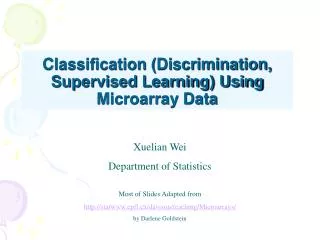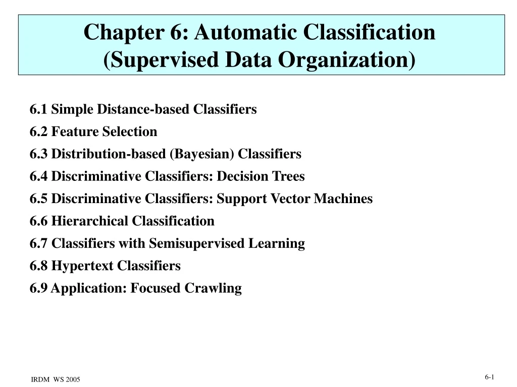

Chapter 6: Automatic Classification (Supervised Data Organization)
E N D
Presentation Transcript
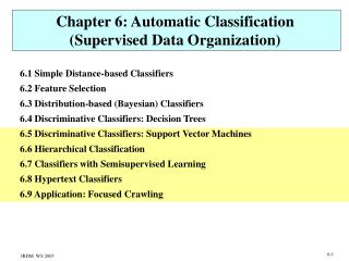
Chapter 6: Automatic Classification(Supervised Data Organization) 6.1 Simple Distance-based Classifiers 6.2 Feature Selection 6.3 Distribution-based (Bayesian) Classifiers 6.4 Discriminative Classifiers: Decision Trees 6.5 Discriminative Classifiers: Support Vector Machines 6.6 Hierarchical Classification 6.7 Classifiers with Semisupervised Learning 6.8 Hypertext Classifiers 6.9 Application: Focused Crawling
f2 f2 f2 f1 f1 f1 Classification Problem (Categorization) given: feature vectors determine class/topic membership(s) of feature vectors known classes + labeled training data: supervised learning unknown classes: unsupervised learning (clustering) ?
Filtering: test newly arriving documents (e.g. mail, news) • if they belong to a class of interest (stock market news, spam, etc.) • Summary/Overview: organize query or crawler results, • directories, feeds, etc. • Query expansion: assign query to an appropriate class and • expand query by class-specific search terms • Relevance feedback: classify query results and let the user • identify relevant classes for improved query generation • Word sense disambiguation: mapping words (in context) to concepts • Query efficiency: restrict (index) search to relevant class(es) • (Semi-) Automated portal building: automatically generate • topic directories such as yahoo.com, dmoz.org, about.com, etc. Uses of Automatic Classification in IR • Classification variants: • with terms, term frequencies, link structure, etc. as features • binary: does a document d belong class c or not? • many-way: into which of k classes does a document fit best? • hierarchical: use multiple classifiers to assign a document • to node(s) of topic tree
Automatic Classification in Data Mining Goal: Categorize persons, business entities, or scientific objects and predict their behavioral patterns • Application examples: • categorize types of bookstore customers based on purchased books • categorize movie genres based on title and casting • categorize opinions on movies, books, political discussions, etc. • identify high-risk loan applicants based on their financial history • identify high-risk insurance customers based on • observed demoscopic, consumer, and health parameters • predict protein folding structure types based on • specific properties of amino acid sequences • predict cancer risk based on genomic, health, and other parameters • ...
WWW / Intranet ...... ..... ...... ..... automatic assignment automatische Zuweisung automatische Zuweisung automatische Zuweisung estimate and assign document to the class with the highest probability e.g. with Bayesian method: training data ... Classification with Training Data(Supervised Learning): Overview Science classes feature space: term frequencies fi (i = 1, ..., m) Mathematics new documents Algebra ... Probability and Statistics Hypotheses Testing Large Deviation ... intellectual assignment
empirical by automatic classification of documents that do not belong to the training data (but in benchmarks class labels of test data are usually known) Assessment of Classification Quality • For binary classification with regard to class C: • a = #docs that are classified into C and do belong to C • b = #docs that are classified into C but do not belong to C • c = #docs that are not classified into C but do belong to C • d = #docs that are not classified into C and do not belong to C Error (Fehler) = 1accuracy Acccuracy (Genauigkeit) = Precision (Präzision) = Recall (Ausbeute) = F1 (harmonic mean of precision and recall) = • For manyway classification with regard to classes C1, ..., Ck: • macro average over k classes or • micro average over k classes
Estimation of Classifier Quality use benchmark collection of completely labeled documents (e.g., Reuters newswire data from TREC benchmark) • cross-validation (with held-out training data): • partition training data into k equally sized (randomized) parts, • for every possible choice of k-1 partitions • train with k-1 partitions and apply classifier to kth partition • determine precision, recall, etc. • compute micro-averaged quality measures leave-one-out validation/estimation: variant of cross-validation with two partitions of unequal size: use n-1 documents for training and classify the nth document
6. 1 Distance-based Classifiers:k-Nearest-Neighbor Method (kNN) Step 1: find among the training documents of all classes the k (e.g. 10-100) most similar documents (e.g., based on cosine similarity): the k nearest neighbors of Step 2: Assign to class Cj for which the function value is maximized With binary classification assign to class C if is above some threshold ( >0.5)
Distance-based Classifiers: Rocchio Method Step 1: Represent the training documents for class Cj by a prototype vector with tf*idf-based vector components with appropriate coefficients and (e.g. =16, =4) Step 2: Assign a new document to the class Cj for which the cosine similarity is maximized.
6.2 Feature Selection • For efficiency of the classifier and to suppress noise • choose subset of all possible features. • Selected features should be • frequent to avoid overfitting the classifier to the training data, • but not too frequent in order to be characteristic. • Features should be good discriminatorsbetween classes • (i.e. frequent/characteristic in one class but infrequent in other classes). • Approach: • compute measure of discrimination for each feature • select the top k most discriminative features in greedy manner tf*idf is usually not a good discrimination measure, and may give undue weight to terms with high idf value (leading to the danger of overfitting)
Example for Feature Selection theorem integral vector Class Tree: group chart limit film hit f1 f2 f3 f4 f5 f6 f7 f8 d1: 1 1 0 0 0 0 0 0 d2: 0 1 1 0 0 0 1 0 d3: 1 0 1 0 0 0 0 0 d4: 0 1 1 0 0 0 0 0 d5: 0 0 0 1 1 1 0 0 d6: 0 0 0 1 0 1 0 0 d7: 0 0 0 0 1 0 0 0 d8: 0 0 0 1 0 1 0 0 d9: 0 0 0 0 0 0 1 1 d10: 0 0 0 1 0 0 1 1 d11: 0 0 0 1 0 1 0 1 d12: 0 0 1 1 1 0 1 0 Entertainment Math Algebra Calculus training docs: d1, d2, d3, d4 Entertainment d5, d6, d7, d8 Calculus d9, d10, d11, d12 Algebra
Simple (Class-unspecific)Criteria for Feature Selection Document Frequency Thresholding: Consider for class Cj only terms ti that occur in at least training documents of Cj. Term Strength: For decision between classes C1, ..., Ck select (binary) features Xi with the highest value of • To this end the set of similar doc pairs (d, d‘) is obtained • by thresholding on pairwise similarity or • by clustering/grouping the training docs. + further possible criteria along these lines
Feature Selection Based on 2 Test For class Cj select those terms for which the 2 test (performed on the training data) gives the highest confidence that Cj and ti are not independent. As a discrimination measure compute for each class Cj and term ti: with absolute frequencies freq
Feature Selection Based on Information Gain Information gain: For discriminating classes c1, ..., ck select the binary features Xi (term occurrence) with the largest gain in entropy can be computed in time O(n)+O(mk) for n training documents, m terms, and k classes
Feature Selection Based on Mutual Information Mutual information (Kullback-Leibler distance, relative entropy): for class cj select those binary features Xi (term occurrence) with the largest value of and for discriminating classes c1, ..., ck: can be computed in time O(n)+O(mk) for n training documents, m terms, and k classes
assess goodness of term „chart (c)“ for discriminating classes „Entertainment (E)“ vs. „Math (M)“ Example for Feature Selection Based on 2, G, and MI base statistics: n=12 training docs; f(E) = 4 docs in E; f(M)=8 docs in M; f(c)=4 docs contain c; f( )=8 docs don‘t contain c; f(cE)=3 docs in E contain c; f(cM)=1 doc in M contains c; f( E)=1 doc in E doesn‘t contain c; f( M)=7 docs in M don‘t contain c; p(c)=4/12=prob. of random doc containing c p(cE)=3/12=prob. of random doc containing c and being in E etc. 2(chart) = (f(cE)-f(c)f(E)/n)2) / (f(c)f(E)/n) + ... (altogether four cases) = (3 – 4*4/12)2 / (4*4/12) + (1 – 4*8/12)2 / (4*8/12) + (1 – 8*4/12)2 / (8*4/12) + (7 – 8*8/12)2 / (8*8/12) G(chart) = p(E) log 1/p(E) + p(M) log 1/p(M) – p(c) ( p(cE) log 1/p(cE) + p(cM log 1/p(cM)) – p( ) ( analogously for ) = 1/3 log3 + 2/3 log3/2 – 4/12 (3/4 log4/3 + 1/4 log4) – 8/12 (1/8 log 8 + 7/8 log 8/7 ) MI(chart) = p(cE) log (p(cE) / (p(c)p(E))) + ... (altogether four cases) = 3/12 log (3/12 / (4*4/144)) + 1/12 log (1/12 / (4*8/144)) + 1/12 log (1/12 / (8*4/144)) + 7/12 log (7/12 / (8*8/144))
For document sets X in class C and Y not in class C find m-dimensional vector that maximizes Feature Selection Based on Fisher Index Fisher‘s discriminant (finds projection that maximizes ratio of projected centroid distance to variance) with covariance matrix: solution requires inversion of For feature selection consider vectors j = (0 ... 0 1 0 ... 0) with 1 at the position of the j-th term and compute Fisher‘s index (FI) (indicates feature contribution to good discrimination vector) Select features with highest FI values
Idea: start with all features F and a drop feature X if there is an approximate Markov blanket M for X in F-{X}: M is a Markov blanket for X in F if X is conditionally independent of F – (M{X}) given M. Feature Space Truncation Using Markov Blankets Algorithm: F‘ := F while distribution P[Ck | F‘] is close enough to original P[Ck | F] do for each X in F‘ do identify candidate Markov blanket M for X (e.g. the k most correlated features) compute KL distance between distributions P[Ck | M {X}] and P[Ck | M] over classes Ck end eliminate feature X with smallest KL distance: F‘ := F – {X} end Advantage over greedy feature selection: considers feature combinations
6.3 Distribution-based Classifiers:Naives Bayes with Binary Features Xi estimate: with feature independence or linked dependence: with empirically estimated pik=P[Xi=1|ck], pk=P[ck] for binary classification with odds rather than probs for simplification
Naive Bayes with Binomial Bag-of-Words Model estimate: with term frequency vector with feature independence with binomial distribution for each feature using ML estimator: satisfying or with Laplace smoothing:
Naive Bayes with Multinomial Bag-of-Words Model estimate: with term frequency vector with feature independence with multinomial distribution of features and constraint with
Example for Naive Bayes 3 classes: c1 – Algebra, c2 – Calculus, c3 – Stochastics 8 terms, 6 training docs d1, ..., d6: 2 for each class p1=2/6, p2=2/6, p3=2/6 Algebra Stochastics Calculus homomorphism k=1 k=2 k=3 p1k 4/12 0 1/12 p2k 4/12 0 0 p3k 3/12 1/12 1/12 p4k 0 5/12 1/12 p5k 0 5/12 1/12 p6k 0 0 2/12 p7k 0 1/12 4/12 p8k 1/12 0 2/12 probability variance integral vector group limit dice f1 f2 f3 f4 f5 f6 f7 f8 d1: 3 2 0 0 0 0 0 1 d2: 1 2 3 0 0 0 0 0 d3: 0 0 0 3 3 0 0 0 d4: 0 0 1 2 2 0 1 0 d5: 0 0 0 1 1 2 2 0 d6: 1 0 1 0 0 0 2 2 without smoothing for simple calculation
Example of Naive Bayes (2) classification of d7: ( 0 0 1 2 0 0 3 0 ) for k=1 (Algebra): for k=2 (Calculus): for k=3 (Stochastics): Result: assign d7 to class C3 (Stochastics)
Typical Behavior of the Naive Bayes Method Reuters Benchmark (see trec.nist.gov): 12902 short newswire articles (business news) from 90 categories (acq, corn, earn, grain, interest, money-fx, ship, ...) • Use (a part of) the oldest 9603 articles for training the classifier • Use the most recent 3299 articles for testing the classifier typical behavior accuracy 1000 3000 6000 9000 # training docs max. accuracy is between 50 and 90 percent (depending on category)
Improvements of the Naive Bayes Method 1) smoothed estimation of the pik values (e.g. Laplace smoothing) 2) classify unlabeled documents and use their terms for better estimation of pik values (i.e., the model parameters) possibly using different weights for term frequencies in real training docs vs. automatically classified docs Section 6.7 on semisupervised classification 3) consider most important correlations between features by extending the approach to a Bayesian net
Framework for Bayes Optimal Classifiers Use any suitable parametric model for the joint distribution of features and classes, with parameters for (assumed) prior distribution (e.g. Gaussian) A classifier for class c that maximizes for given test document d and training data D is called Bayes optimal
Maximum Entropy Classifier • Approach for estimating : • estimate parameters of probability distribution such that • the expectations Eik for all features fi and classes Ckmatch the • empirical mean values Mik (derived from n training vectors) and • have maximum entropy (i.e. postulate uniform distribution • unless the training data indicate a different distribution) • distribution has loglinear form • with normalization constant Z: Compute parameters i by iterative procedure (generalized iterative scaling), which is guaranteed to converge under specific conditions
6.4 Discriminative Classifiers: Decision Trees given: a multiset of m-dimensional training data records dom(A1) ... dom(Am) with numerical, ordinal, or categorial attributes Ai (e.g. term occurrence frequencies N0 ... N0) and with class labels • wanted: a tree with • attribute value conditions of the form • Ai value for numerical or ordinal attributes • or • Ai value set or Ai value set = • for categorial attributes • or • linear combinations of this type • for several numerical attributes • as inner nodes and • labeled classes as leaf nodes
Examples for Decision Trees (1) tf(homomorphism) 2 has read Tolkien T F T F tf(vector) 3 tf(limit) 2 has read Eco boring T F T F T F intellectual uneducated Lineare Algebra Algebra Calculus Other salary 100000 T F university degree & salary 50000 credit worthy T F credit worthy not credit worthy
Examples for Decision Trees (2) vertebrate work time 60 hours/week T T F ... #legs 2 hobbies {climbing, paragliding} hobbies {paragliding} T ... skin {scaly, leathery} T F T F T high risk normal high risk normal ... snakes weather forecast sunny rainy cloudy wind humidity high normal strong weak no golf golf golf golf no golf
Top-Down Construction of Decision Tree Input: decision tree node k that represents one partition D of dom(A1) ... dom(Am) Output: decision tree with root k • BuildTree (root, dom(A1) ... dom(Am)) • PruneTree: reduce tree to appropriate size • with: • procedure BuildTree (k, D): • if k contains only training data of the same class then terminate; • determine split dimension Ai; • determine split value x for most suitable partitioning of D into • D1 = D{d | d.Ai x} and D2= D{d | d.Ai > x}; • create children k1 and k2 of k; • BuildTree (k1, D1); BuildTree (k2, D2);
Split Criterion Information Gain Goal is to split current node such that the resulting partitions are as pure as possible w.r.t. class labels of the corresponding training data. Thus we aim to minimize the impurity of the partitions. An approach to define impurity is via the entropy-based (statistical) information gain (referring to the distribution of class labels within a partition) G (k, k1, k2) = H(k) – ( p1*H(k1) + p2*H(k2) ) where: nk: # training data records in k nk,j: # training data records in k that belong to class j p1 = nk1 / nk and p2 = nk2 / nk
Alternative Split Criteria 1) split such that the entropy of k1 and k2 is minimized: p1*H(k1) + p2*H(k2) 2) split such that GI(k1)+GI(k2) is minimized with the „Gini index“: 3) The information gain criterion prefers branching by attributes with large domains (many different values) Alternative: split criterion information gain ratio
Problem: complete decision trees with absolutely pure leaf nodes tend tooverfitting – branching even in the presence of rather insignificant training data („noise“): this minimizes the classification error on the training data, but may not generalize well to new test data Criteria for Tree Pruning • Solution: remove leaf nodes until only significant branching nodes • are left, using the principle of • Minimum Description Length (MDL): • describe the class labels of all training data records • with minimal length (in bits) • K bits per tree node (attribute, attribute value, pointers) • nk*H(k) bits for explicit class labels of all • nk training data records of a leaf node k with
Example for Decision Tree Construction (1) Training data: weather temperature humidity wind golf forecast 1) sunny hot high weak no 2) sunny hot high strong no 3) cloudy hot high weak yes 4) rainy mild high weak yes 5) rainy cold normal weak yes 6) rainy cold normal strong no 7) cloudy cold normal strong yes 8) sunny mild high weak no 9) sunny cold normal weak yes 10) rainy mild normal weak yes 11) sunny mild normal strong yes 12) cloudy mild high strong yes 13) cloudy hot normal weak yes 14) rainy mild high strong no
Example for Decision Tree Construction (2) weather forecast G: 9, no G: 5 sunny cloudy rainy ? Golf ? G: 3, no G: 2 G: 4, no G: 0 G: 2, no G: 3 data records: 1, 2, 8, 9, 11 entropy H(k): 2/5*log25/2 + 3/5*log25/3 2/5*1.32 + 3/5*0.73 0.970 choice of split attribute: G(humidity): 0.970 – 3/5*0 – 2/5*0 = 0.970 G(temperature): 0.970 – 2/5*0 – 2/5*1 – 1/5*0 = 0.570 G(wind): 0.970 – 2/5*1 –3/5*0.918 = 0.019
homomorphism probability. variance integral vector group limit dice f1 f2 f3 f4 f5 f6 f7 f8 d1: 3 2 0 0 0 0 0 1 d2: 1 2 3 0 0 0 0 0 d3: 0 0 0 3 3 0 0 0 d4: 0 0 1 2 2 0 1 0 d5: 0 0 0 1 1 2 2 0 d6: 1 0 1 0 0 0 2 2 Example for Decision Tree for Text Classification C1: Algebra C2: Calculus C3: Stochastics f2>0 G = H(k) – ( 2/6*H(k1) + 4/6*H(k2) ) H(k) = 1/3 log 3 + 1/3 log 3 + 1/3 log 3 H(k1) = 1 log 1 + 0 + 0 H(k2) = 0 + 1/2 log 2 + 1/2 log 2 G = log 3 – 0 – 2/3*1 1,6 – 0,66 = 0,94 f7>1 Algebra Stochastics Calculus
Example for Decision Tree Pruning 3 classes: C1, C2, C3 100 training data records C1: 60, C2: 30, C3: 10 A < ... C1: 45 C2: 10 C3: 5 B < ... C < ... D < ... E < ... F < ... G < ... C1: 45 C2: 5 C2:5 C3:5 C1:45 C2:5 C2:5 C3:5 Assumption: coding cost of a tree node is K=30 bits coding cost of D subtree: 50*(0.9 log210/9 + 0.1 log210) 50*(0.9*0.15 + 0.1*3.3) 50*0.465 < 30 coding cost of E subtree: 10*(0.5*log22 + 0.5*log22) = 10 < 30 coding cost of B subtree: 60*(9/12*log212/9 + 1/6*log26 + 1/12*log212) 60*(0.75*0.4 + 0.166*2.6 + 0.083*3.6) > 30
Problems of Decisison Tree Methodsfor Classification of Text Documents • Computational cost for training is very high. • With very high dimensional, sparsely populated feature spaces • training could easily lead to overfitting.
Rule Induction (Inductive Logic Programming) represents training data as simple logic formulas such as: faculty (doc id ...) student (doc id ...) contains (doc id ..., term ...) ... aims to generate rules for predicates such as: contains (X, „Professor“) faculty (X) contains (X, „Hobbies“) & contains (X, „Jokes“) student (X) and possibly generalizing to rules about relationships such as: link(X,Y) & link(X,Z) & course(Y) & publication(Z) faculty(X) generates rules with highest confidence driven by frequency of variable bindings that satisfy a rule Problem: high complexity and susceptible to overfitting
Classification and Feature-Selection Models and Algorithms: • S. Chakrabarti, Chapter 5: Supervised Learning • C.D. Manning / H. Schütze, Chapter 16: Text Categorization, • Section 7.2: Supervised Disambiguation • J. Han, M. Kamber, Chapter 7: Classification and Prediction • T. Mitchell: Machine Learning, McGraw-Hill, 1997, • Chapter 3: Decision Tree Learning, Chapter 6: Bayesian Learning, • Chapter 8: Instance-Based Learning • D. Hand, H. Mannila, P. Smyth: Principles of Data Mining, MIT Press, 2001, • Chapter 10: Predictive Modeling for Classification • M.H. Dunham, Data Mining, Prentice Hall, 2003, Chapter 4: Classification • M. Ester, J. Sander, Knowledge Discovery in Databases, Springer, 2000, • Kapitel 4: Klassifikation • Y. Yang, J. Pedersen: A Comparative Study on Feature Selection in • Text Categorization, Int. Conf. on Machine Learning, 1997 • C.J.C. Burges: A Tutorial on Support Vector Machines for Pattern Recognition, • Data Mining and Knowledge Discovery 2(2), 1998 • S.T. Dumais, J. Platt, D. Heckerman, M. Sahami: Inductive Learning • Algorithms and Representations for Text Categorization, CIKM Conf. 1998 Additional Literature for Chapter 6