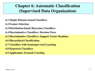
Chapter 6: Automatic Classification (Supervised Data Organization)
Chapter 6: Automatic Classification (Supervised Data Organization). 6.1 Simple Distance-based Classifiers 6.2 Feature Selection 6.3 Distribution-based (Bayesian) Classifiers 6.4 Discriminative Classifiers: Decision Trees 6.5 Discriminative Classifiers: Support Vector Machines

Chapter 6: Automatic Classification (Supervised Data Organization)
E N D
Presentation Transcript
Chapter 6: Automatic Classification(Supervised Data Organization) 6.1 Simple Distance-based Classifiers 6.2 Feature Selection 6.3 Distribution-based (Bayesian) Classifiers 6.4 Discriminative Classifiers: Decision Trees 6.5 Discriminative Classifiers: Support Vector Machines 6.6 Hierarchical Classification 6.7 Classifiers with Semisupervised Learning 6.8 Hypertext Classifiers 6.9 Application: Focused Crawling
x2 x1 6.5 Discriminative Classifiers: Support Vector Machines (SVM) for Binary Classification n training vectors (x1, ..., xm, C) with C = +1 or -1 ? C C large-margin separating hyperplane minimizes risk of classification error Determine hyperplane that optimally separates the training vectors in C from those not in C, such that the (Euclidean) distance of the (positive and negative) training samples closest to the hyperplane is maximized. (Vectors with distance are called support vectors.) Classify new test vector into C if:
Find and b R such that • R is maximal and • for all i=1, ..., n Computation of the Optimal Hyperplane This is (w.l.o.g. with the choice ) equivalent to (V. Vapnik: Statistical Learning Theory, 1998): • Find such that • is minimal • and (Quadratic programming problem) Optimal vector ist linear combination (where i > 0 only for support vectors) b is derived from any support vector by:
x2 x1 SVMs with Nonlinear Separation C C C Transform vectors into with m‘ > m e.g.: C and C could then be linearly separable in the m‘-dimensional space For specific with a kernel function both training and classification remain efficient, e.g. for the family of polynoms classification test for new vector :
SVM Kernels • Popular and well-understood kernel functions: • polynomial kernels: • radial basis function • (Gaussian kernel): • neural network • (sigmoid function): • string kernels etc. • (e.g., for classification of biochemical sequences)
x2 x1 SVMs with “Soft” Separation If training data are not completely separable tolerate a few „outliers“ on the wrong side of the hyperplane • Find and b R such that • is minimal and • for all i=1, ..., n with control parameter for trading off separation margin vs. error sum
SVM Engineering + Very efficient implementations available (e.g., SVM-Light at http://svmlight.joachims.org/): with training time empirically found to be quadratic in # training docs (and linear in # features) + SVMs can and should usually consider all possible features (no point for feature selection unless #features intractable) + multi-class classification mapped to multiple binary SVMs: one-vs.-all or combinatorial design of subset-vs.-complement Choice of kernel and soft-margin parameter difficult and highly dependent on data and application: high minimizes training error, but leads to poor generalization (smaller separation, thus higher risk)
6.6 Hierarchical Classification given: tree of classes (topic directory) with training data for each leaf or each node wanted: assignment of new documents to one or more leaves or nodes Top-down approach 1 (for assignment to exactly one leaf): Determine – from the root to the leaves – at each tree level the class into which the document suits best. Top-down approach 2 (for assignment to one or more nodes): Determine – from the root to the leaves – at each tree level those classes for which the confidence in assigning the document to the class lies above some threshold.
Feature Selection for Hierarchical Classification Features must be good discriminators between classes with the same parent feature selection must be „context-sensitive“ • Examples: • Terms such as „Definition“, „Theorem“, „Lemma“ are good discriminators • between Arts, Entertainment, Science, etc. • or between Biology, Mathematics, Social Sciences, etc.; • they are poor discriminators • between subclasses of Mathematics such as Algebra, Stochastics, etc. • The word „can“ is usually a stopword, • but it can be an excellent discriminator • for the topic /Science/Environment/Recycling. Solution: consider only „competing“ classes with the same parent when using information-theoretic measures for feature selection (see Section 6.2)
Example for Feature Selection theorem integral vector Class Tree: group chart limit film hit f1 f2 f3 f4 f5 f6 f7 f8 d1: 1 1 0 0 0 0 0 0 d2: 0 1 1 0 0 0 1 0 d3: 1 0 1 0 0 0 0 0 d4: 0 1 1 0 0 0 0 0 d5: 0 0 0 1 1 1 0 0 d6: 0 0 0 1 0 1 0 0 d7: 0 0 0 0 1 0 0 0 d8: 0 0 0 1 0 1 0 0 d9: 0 0 0 0 0 0 1 1 d10: 0 0 0 1 0 0 1 1 d11: 0 0 0 1 0 1 0 1 d12: 0 0 1 1 1 0 1 0 Entertainment Math Algebra Calculus training docs: d1, d2, d3, d4 Entertainment d5, d6, d7, d8 Calculus d9, d10, d11, d12 Algebra
Experimental Results on HierarchicalText Classification (1) ca. 400 000 documents (from www.looksmart.com) from ca. 17000 classes in 7 levels: 13 classes at level 1 (Automotive, Business&Finance, Computers&Internet, Entertainment&Media, Health&Fitness, etc.), 150 classes at level 2 ca. 50 000 randomly chosen documents as training data; for each of the 13+150 classes selection of 1000 terms with the highest mutual information MI(X,C) Automatic classification of 10 000 documents with SVM (with control parameter =0.01): Top-down assignment of a document to all classes for which the distance to the separating hyperplane was above some threshold (with experimentally chosen so as to maximize classification quality for training data ) from: S. Dumais, H. Chen. Hierarchical Classification of Web Content. ACM SIGIR Conference on Research and Development in Information Retrieval, Athens, 2000
Experimental Results on HierarchicalText Classification (2) Micro-averaged classification quality (F1 measure) level 1 (13 classes): F1 0.572 level 2 (150 classes): F1 0.476 Best and worst classes: F1 0.841 Health & Fitness / Drugs & Medicine F1 0.797 Home & Family / Real Estate F1 0.841 Reference & Education / K-12 Education F1 0.841 Sports & Recreation / Fishing F1 0.034 Society & Politics / World Culture F1 0.088 Home & Family / For Kids F1 0.122 Computers & Internet / News & Magazines F1 0.131 Computers & Internet / Internet & the Web from: S. Dumais, H. Chen. Hierarchical Classification of Web Content. ACM SIGIR Conference on Research and Development in Information Retrieval, Athens, 2000
Handling Classes with Very Few Training Docs Problem: classes at or close to leaves may have very few training docs Idea: exploit feature distributions from ancestor classes • Shrinkage procedure: • Consider classification test of doc d against class cn • with class path c0 (= root = all docs) c1 ... cn • and assume that classifiers use parameterized probability model • with (ML) estimators ci,t for class ci and feature t • For ci classifier instead of using ci,t • use „shrunk“ parameters: • where • Determine i values by iteratively improving accuracy • on held-out training data
6.7 Classifiers with Semisupervised Learning • Motivation: • classifier can only be as good as its training data • and training data is expensive to obtain as it • requires intellectual labeling • and training data is often sparse regarding the feature space • use additional unlabeled data to improve the classifier‘s • implicit knowledge of term correlations • Example: • classifier for topic „cars“ has been trained only with documents • that contain the term „car“ but not the term „automobile“ • in the unlabeled docs of the corpus the terms • „car“ and „automobile“ are highly correlated • test docs may contain the term „autombobile“ but not the term „car“
Simple Iterative Labeling Let DK be the set of docs with known labels (training data) and DU the set of docs with unknown labels. Algorithm: train classifier with DKas training data classify docs in DU repeat re-train classifier with DK and the now labeled docs in DU classify docs in DU until labels do not change anymore (or changes are marginal) Robustness problem: a few misclassified docs from DU could lead the classifier to drift to a completely wrong labeling
EM Iteration (Expectation-Maximization) Idea [Nigam et al. 2000]: E-step: assign docs from DU to topics merely with certain probabilities M-step: use these probabilities to better estimate the model‘s parameters • Algorithm (for Bayesian classifier): • train classifier with DK as training data • E-step: compute probabilities P[Ck | d] for all d in DU • repeat • M-step: estimate parameters pik of the Bayesian model • (optionally with Laplace smoothing, or using MLE) • E-step: recompute probabilities P[Ck | d] for all d in DU • until changes of max(P[Ck | d] | k=1..#classes) become marginal • assign d from DU to argmaxk(P[Ck | d])
Experimental Results [Nigam et al. 2000] accuracy # training docs
Co-Training for Orthogonal Feature Spaces • Idea: • start out with two classifiers A and B for „orthogonal“ feature spaces • (whose distributions are conditionally independent given the class labels) • add best classified doc of A to training set of B, and vice versa • (assuming that the same doc would be given the same label by A and B) Algorithm: train A and B with orthogonal features of DK (e.g., text terms and anchor terms) DUA:= DU; DUB:= DU;DKA:= DK; DKB:= DK; repeat classify docs in DUA by A and DUB by B select the best classified docs from DUA and DUB: dA and dB add dA to training set DKB, add dB to training set DKA retrain A using DKA, retrain B using DKB until results are sufficiently stable assign docs from DU to classes on which A and B agree
More Meta Strategies Combine multiple classifiers for more robust results (usually higher precision and accuracy, possibly at the expense of reduced recall) Examples (with m different binary classifiers for class k): • unanimous decision: • weighted average: with precision estimator for classifier for further info see machine learning literature on ensemble learning (stacking, boosting, etc.)
6.8 Hypertext Classifiers • Motivation: • the hyperlink neighbors of a test document may exhibit information • that helps for the classification of the document • Examples: • the test document is referenced (only) by a Web page that contains • a highly specific keywords that are not present in the document itself • (e.g. the word „soccer“ in a page referencing the results of • last week‘s Champions League matches) • the test document is referenced by a Web page that is listed under a • specific topic in a manually maintained topic directory • (e.g. the topic „sports“ in page referencing the results of ...) • the test document is referenced by a Web page that also references • many training documents for a specific topic
Using Features of Hyperlink Neighbors Idea: consider terms and possibly class labels of hyperlink neighbors Approach 1: extend each document by the terms of its neighbors (within some hyperlink radius R and possibly with weights ~ 1/r for hyperlink distance r) Problem: susceptible to „topic drift“ Example: Link from IRDM course page to www.yahoo.com Approach 2: when classifying a document consider the class labels of its neighbors
Consideration of Neighbor Class Labels Typical situation: c1: Arts ... c1: Arts c2: Music test doc. topic- specific hub class un- known di c1: Arts c3: Enter- tain- ment c2: Music ... unspecific portal ... c4: Computer
Neighborhood-conscious Feature Space Construction ? sports ? golden goal seminfinal Turkey Ronaldo goal politics Völler Kahn match final Brazil Yokohama Schröder Yokohama Japan Yen sports sports world champion Brazil Germany Brazil consider known class labels of neighboring documents
Neighborhood-conscious Feature Space Construction 0.8 sports 0.2 politics ? ? golden goal seminfinal Turkey 0.7 politics 0.3 sports Ronaldo goal Völler Kahn match final Brazil Yokohama 0.8 sports 0.2 politics Schröder Yokohama Japan Yen 0.6 sports 0.4 politics world champion Brazil Germany Brazil consider known class labels of neighboring documents consider term-based class probabilities of neighboring documents
Neighborhood-conscious Feature Space Construction ? ? ? golden goal seminfinal Turkey Ronaldo goal ? Völler Kahn match final Brazil Yokohama Schröder Yokohama Japan Yen ? ? world champion Brazil Germany Brazil consider known class labels of neighboring documents consider term-based class probabilities of neighboring documents evaluate recurrence between class prob. distr. of all documents: iterative relaxation labeling for Markov random field
Relaxation labeling in action ? ? ? ? Marginal distributions: .5 Blue .5 Green ? ? Citation matrix ? ?
Relaxation labeling in action ? ? ? ? Marginal distributions: .5 Blue .5 Green ? ? Citation matrix ? ?
Relaxation labeling in action ? ? ? ? Marginal distributions: .5 Blue .5 Green ? ? Citation matrix ? ?
Simple Iterative Labelingwith Exploitation of Neighbor Class Labels • for all docs d with unknown class • classify d using the terms of d • Repeat • train classifier that exploits class labels of neighbors • of all docs d with originally unknown class • classify d using the extended classifier • that exploits neighbor labels • until labels do not change anymore (or changes are marginal)
Naive Bayes Classifier withConsideration of Neighbor Class Labels analyze or conditional independence assumptions with pred(di) := {dj | (j, i)E} and succ(di) := {dj | (i, j)E}
Digression: Markov Random Fields (MRFs) Let G = (V, E) be an undirected graph with nodes V and edges E. The neighborhood N(x) of xV is {y V | (x,y) E}. All neighborhoods together form a neighborhood system. Associate with each node vV a random variable Xv. A probability distribution for (Xv1, ..., Xvn) with V={v1, ..., vn} is called a Markov random field w.r.t. the neighborhood system on G if for all Xvi the following holds: for MRF theory see, for example, the book: S.Z. Li, Markov Random Field Modeling in Image Analysis, 2001..
Naive Bayes Classifier with Considerationof Unknown Class Labels of Neighbors (1) with known class labels of neighbors: assign di to class ck for which f(ck, di, Ni) is maximal with (partly) unknown class labels of neighbors apply Iterative Relaxation Labeling: construct neighborhood graph Gi=(Ni,Ei) with radius R around di; classify all docs in Ni based on text features; repeat for all dj in Ni (incl. di) do compute the class label of dj based on text features of dj and the class label distribution of Nj using Naive Bayes end; until convergence is satisfactory
Naive Bayes Classifier with Considerationof Unknown Class Labels of Neighbors (2) Divide neighbor documents of di into NiK – docs with known class labels and NiU – docs with a priori unknown class labels. Let K be the union of docs NjKwith known labels for all considered dj. Then: with the set i of all possible class labelings c of Ni for convergence conditions of Iterative Relaxation Labeling see theory of MRFs
Experimental Resultson Hypertext Classification (1) ca. 1000 patents from 12 classes: Antenna, Modulator, Demodulator, Telephony, Transmission, Motive, Regulator, Heating, Oscillator, Amplifier, Resistor, System. classification accuracy with text features alone: 64% classification accuracy with hypertext classifier: 79% ca. 20000 Web documents from 13 Yahoo classes: Arts, Business&Economy, Computers&Internet, Education, Entertainment, Government, Health, Recreation, Reference, Regional, Science, Social Science, Society&Culture. classification accuracy with text features alone: 32% classification accuracy with hypertext classifier: 79% from: S. Chakrabarti, B. Dom, P. Indyk. Enhanced Hypertext Categorization Using Hyperlinks. ACM SIGMOD International Conference on Management of Data, Seattle, 1998.
Experimental Resultson Hypertext Classification (2) accuracy % of neighbors with a priori known class labels from: S. Chakrabarti, B. Dom, P. Indyk. Enhanced Hypertext Categorization Using Hyperlinks. ACM SIGMOD International Conference on Management of Data, Seattle, 1998.
Extended Techniques for Graph-based Classification • neighbor pruning: • consider only neighbors with content similarity above threshold • (effectively remove edges) • edge weighting: • capture confidence in neighbors (e.g. content similarity) • by edge weights, • and use weights in class-labeling probabilities • recompute neighbor-class-pair probabilities in each RL iteration • incorporate relationship strengths between different class labels
Cost-based Labeling for simplicity consider only two classes C and C given:marginal distribution of classes: P[dX] with X = C or X = C and class citation probability distribution: P[dj X | di references dj di Y] with X, Y being C or C find:assignment of class labels x1, ..., xn to documents d1, ..., dn DU s.t. P[d1x1 ... dn xn | DK] is maximized approach: minimize log P[d1x1 ... dn xn | DK] = ilog P[di xi | DK] assuming independence NP-complete problem, but with good approximation algorithms. see: J. Kleinberg, E. Tardos, Approximation Algorithms for Classification Problems with Pairwise Relationships: Metric Labeling and Markov Random Fields, Journal of the ACM Vol.49 No.5, 2002.
WWW ...... ..... ...... ..... • critical issues: • classifier accuracy • feature selection • quality of training data 11.9 Application: Focused Crawling automatially build personal topic directory seeds Crawler training Classifier Link Analysis Root DB Core Technology Semistrutured Data Web Retrieval Data Mining XML
WWW ...... ..... ...... ..... Root DB Core Technology Semistrutured Data Web Retrieval Data Mining XML The BINGO! Focused Crawler seeds Crawler training Classifier Link Analysis high SVM confidence high HITS authority score re-training topic-specific archetypes
BINGO! Adaptive Re-trainingand Focus Control for each topic V do { archetypes(V) := top docs of SVM confidence ranking top authoritiesof V ; remove from archetypes(V) all docs d that do not satisfy confidence(d) mean confidence(V) ; recompute feature selection based on archetypes(V) ; recompute SVM model for V with archetypes(V)as training data } combine re-training with two-phase crawling strategy: • learning phase: • aims to find archetypes (high precision) • hard focus for crawling vicinity of training docs • harvesting phase: • aims to find results (high recall) • soft focus for long-range exploration with tunnelling
Summary of Chapter 6 • Automatic classification has numerous applications • Naive Bayes, decision trees, SVMs are mature methods • Danger of overfitting: aim for balance between • training error and generalization • may require feature selection • or tuning of regularization parameters • Semisupervised classifiers aim to address training bottleneck • Model selection (parameters, feature engineering) is crucial • Graph-awareness is promising form of richer features
Classification and Feature-Selection Models and Algorithms: • S. Chakrabarti, Chapter 5: Supervised Learning • C.D. Manning / H. Schütze, Chapter 16: Text Categorization, • Section 7.2: Supervised Disambiguation • J. Han, M. Kamber, Chapter 7: Classification and Prediction • T. Mitchell: Machine Learning, McGraw-Hill, 1997, • Chapter 3: Decision Tree Learning, Chapter 6: Bayesian Learning, • Chapter 8: Instance-Based Learning • D. Hand, H. Mannila, P. Smyth: Principles of Data Mining, MIT Press, 2001, • Chapter 10: Predictive Modeling for Classification • M.H. Dunham, Data Mining, Prentice Hall, 2003, Chapter 4: Classification • M. Ester, J. Sander, Knowledge Discovery in Databases, Springer, 2000, • Kapitel 4: Klassifikation • Y. Yang, J. Pedersen: A Comparative Study on Feature Selection in • Text Categorization, Int. Conf. on Machine Learning, 1997 • C.J.C. Burges: A Tutorial on Support Vector Machines for Pattern Recognition, • Data Mining and Knowledge Discovery 2(2), 1998 • S.T. Dumais, J. Platt, D. Heckerman, M. Sahami: Inductive Learning • Algorithms and Representations for Text Categorization, CIKM Conf. 1998 Additional Literature for Chapter 6
Additional Literature for Chapter 6 • Advanced Topics (Semisupervised C., Graph-aware C., Focused Crawling, MDL, etc.): • S. Chakrabarti, Chapter 6: Semisupervised Learning • K. Nigam, A. McCallum, S. Thrun, T. Mitchell: Text Classification from • Labeled and Unlabeled Data Using EM, Machine Learning 39, 2000 • S. Chakrabarti, B. Dom, P. Indyk: Enhanced Hypertext Categorization • Using Hyperlinks, ACM SIGMOD Conference 1998 • S. Chakrabarti, M. van den Berg, B. Dom: Focused crawling: a new • approach to topic-specific Web resource discovery, WWW Conf., 1999 • S. Sizov et al.: The BINGO! System for Information Portal Generation • and Expert Web Search, CIDR Conference, 2003 • S. Siersdorfer, G. Weikum: Using Restrictive Classification and • Meta Classification for Junk Elimination, ECIR 2005 • M. H. Hansen, B. Yu: Model Selection and the Principle of Minimum Description Length, Journal of the American Statistical Association 96, 2001 • P.Grünwald, A Tutorial introduction to the minimum description length principle Advances in Minimum Description Length, MIT Press, 2005