Download

1 / 36
360 likes | 541 Views
Internet Tomography. Bin Yu Statistics Department, UC Berkeley. Collaborators. J. Cao, D. Davis, S. Vander Wiel, G. Liang, R. Castro, M. Coates, A. Hero, R. Nowak, N. Taft. Related papers: Cao, Davis, Vander Wiel, and Yu (JASA, 2000), Coates, Hero, Nowak, and Yu (SPM, 2001)

E N D
Internet Tomography Bin Yu Statistics Department, UC Berkeley
Collaborators J. Cao, D. Davis, S. Vander Wiel, G. Liang, R. Castro, M. Coates, A. Hero, R. Nowak, N. Taft. Related papers: Cao, Davis, Vander Wiel, and Yu (JASA, 2000), Coates, Hero, Nowak, and Yu (SPM, 2001) Liang and Yu (IEEE-SP, 2003), Castro, Coates, Liang, Nowak, and Yu (Statist. Sci., 2004), Liang, Yu, and Taft (Proc. ISIT04).
Medical Tomography • Computer assisted tomography (CAT scanning) • Positron emission tomography (PET scanning) • Single photon emission tomography (SPECT scanning) • All are inverse problems…
Network Tomography The term network tomography was first used by Vardi (1996) to capture the similarities between origin destination (OD) matrix estimation through link counts and medical tomography: in network inference, it is common that one does not observe quantities of interest but their aggregations instead and this goes beyond OD estimation. Vardi (1996) also devised the linear tomography Poisson model for OD traffic estimation and the linear form (not the Poisson assumption) is shown later to approximate other network tomography problems (cf. Coates, Nowak, Hero and Yu, 2002).
Why Network Tomography (NT)? • Network monitoring and management need • - Link packet loss probability • - Link delay • - Origin-Destination (OD) traffic matrix • - Topology/connectivity discovery • - Intrusion detection and prevention • - ... • They are not easily measured directly, but easily measurable indirectly. • Network engineering and resource allocation include • - Routing optimization (OD information needed) • - Quality of service guarantee • - …
NT Example 1: Multicast Link Delay Estimation Probes are sent from the root of a multicasting tree (where routers duplicate the probes and send them to its downstream routers) and delays (Y) are observed at the receiver nodes only. The problem is to infer the distribution of internal links delay (X). Obviously, we have Y=AX, where 1's in the ithrow of A specify the links that the ith component Y travels through.
NT Example 2: OD Traffic Matrix Estimation • n = 4 edge nodes, 1 router, J=8, I=16. • J = n2 = 16 OD pairs in X • I = 7 independent links in Y dst-corp 4 dst-fddi 1 dst-switch 2 dst-local 3 total 4 1 4 2 4 3 4 44 orig-corp 3 1 3 2 3 3 3 43 orig-local 2 1 2 2 2 3 2 42 orig-switch 1 1 1 2 1 3 1 41 orig-fddi
General Linear Network Tomography Model • At a given time t, • X :unknown quantity of interest (of dim J) • (e.g, link delay, traffic flow counts). • Y : known aggregations of X(of dim I). • Problem: predict or estimate X from Y with • AX = Y, • where A is a 0-1 routing matrix. Usually the number J of unknowns is much larger than number I of knowns, so it is a badly ill-posed linear inverse problem. • The special case of OD traffic matrix estimation is of most interest because of its importance to major service providers such as Sprint and AT&T.
Heuristics to Recover X from Y. • Key observations: • Due to the variability in the traffic, covariance of the Y or link measurements give hints on how to attribute traffic to the different OD pairs. • The mean traffic level is related to the variance of the traffic.
Roadmap for OD Estimation • Gaussian Model with Mean-Variance Relationship • Maximum Likelihood Estimation (MLE) for Parameters • Iterative Proportional Fitting (IPF) for OD Traffic Estimation based on Parameter Estimation • Maximum Pseudo-Likelihood Estimation (MPLE) for Parameters • Sprint European Network Data Analysis • A Geometric View: MPLE + IPF vs. Gravity Model + MMI • New: A Partial Measurement Approach (APMA)
Basic Model (Cao et al, 2000) • OD: • Link: • Where • is the unknown parameter, and : positive scale parameter : unknown mean parameter c: power of variance growth with mean, fixed • Variance relation to mean accounts for variations beyond Poisson (c=1 and =1). • The Gaussian mean-variance model was verified in Cao et al (2000) using LAN validation data and recently verified using Sprint European backbone validation data by Melinda et al (2002) and Global Crossing European and American backbone validation data by Gunnar et al (2004).
A Heuristic Identifiability Proof Theorem: is identifiable for fixed c. For the ithorigin-destination pair, : link count at the origin interface : link count at the destination interface. The only bytes that contribute to both of these counts are those from the ith OD pair, and thus implying that i is determined up to the scale . Additional information from E(Y) identifies the scale and identifiability follows. This proof formalizes the idea of using covariances between links motivated by the router 1 traffic plots.
Maximum Likelihood Estimate (MLE) for Gaussian Model Given observed data , the log-likelihood function is Because is functionally related to , no analytic solution to maximize the above expression in terms of : Expectation-Maximization algorithm is used. MLE computation with EM is too slow for large networks.Each EM step has complexity with sparsity matrix calculations. (Cao et al. 2000).
Iterative Proportional Fitting (IPF) for OD Estimation Given Initial Parameter Estimation Given (a) a set of summation linear constraints L (AX=Y) (b) a starting distribution q for X (e.g. MLE estimates for mean OD traffic) I-projection of q to L is Maximum Entropy Principle is a special case when q is uniform. Pythagorean equality: Iterative Proportional Fitting (IPF): a simple alternating minimization procedure to find the I-projection.
Moving Windows to Address Nonstationarity • Dealing with nonstationarity: • Local Likelihood is formed based on n observations such that • Data inside each moving window is assumed to be i.i.d; • Moving windows are overlapping; • Estimates from previous window as starting values for next one. (n=7)
Replacing MLE by Maximum Pseudo-Likelihood Estimation (MPLE) (Liang and Yu, 2003, IEEE-SP) • In order to overcome the computational difficulty of MLE for Markov random field (MRF) inference problems, Besag (1974) proposed a pseudo likelihood (PL) approach. • Sub-problems are formed by neighborhood decomposition; • Pseudo likelihood function is obtained by multiplying the conditional likelihoods from sub-problems, ignoring dependences among sub-problems. • Our pseudo likelihood • has a different scheme for forming sub-problems by using pairs of links and • multiplies likelihoods based on pairs instead of conditional likelihood. • But they share the same divide-and-conquer principle.
MPLE computation • In our experiments, we use sub-problems of all pairs. • The pseudo-EM algorithm is similar to the one used in Cao et al (2000), and the same initial values are used. • The only difference is in E-step: many small matrix inversions instead of one big matrix inversion, and they can be made parallel. • If the average length of OD paths is , then the complexity of one pseudo-EM step is . • Recall that the EM step of MLE has complexity with sparsity matrix calculations. (Cao et al. 2001).
Computation Time Comparison for MLE and MPLE Using network simulator ns, we simulated two networks of 8 end nodes and 21 end nodes, based on the Lucent network topology. For estimating the traffic counts, the computation times (in seconds) are as follows (using R and a 1GHz laptop): # nodes # links MLE MPLE MPLE/MLE 4 7 48 12 0.25 8 16 82 18 0.21 21 49 2300 149 0.06
Sprint Europe Network Data With Validation (OD Traffic Known) Configuration: 13 PoPs, 18 internal links. • Directly measured OD traffic, X, through Cisco’s Netflow • Automatic 10 minute aggregation
Two Sample OD Traffic Plots • Periodicity • Slow-variability of mean OD traffic • Smoothness (nonburstiness), most of time
Cumulative Distribution Plot of Relative Errors Average relative errors: pseudo+IPF is 0.279 and gravity+MMI: 0.305 for large OD traffic.
Boxplot of Relative Errors Boxplot of relative errors for large OD traffic: pseudo+IPF (red) and gravity+MMI (black). All traffic is binned into 10 equal spaced levels.
Gunnar et al (2004) compares different tomographic methods Global Crossing validation data sets: a. European network: 12 PoPs (132 OD pairs), 72 Links ATT approach and variants give best results: about 10% relative error for 29 largest OD pairs (90% total traffic). Worst case bound (LP programming) also gives comparable results. b. American network: 25 PoPs (600 OD pairs), 284 links. ATT approach and variants give best results: 25%. WCB gives 39% for 155 largest OD pairs. Both OD problems are much more well-posed than the Sprint data set.
…. APMA: a partial measurement approach • Liang et al (2004). Proc. ISIT, June. • Rationale: • Direct measurements of OD pairs through NetFlow are becoming available but still computationally expensive. We propose to trade off computation with OD information gathering through: • APMA Algorithm: • For each t, select some OD pairs to measure; • ii) Plug measured OD pairs into AX=Y and use IPF to obtain the remaining X’s with initial values for these X’s estimated from t-1. Recently, Papagiannaki et al (2004) uses complete OD information measured every few days to estimate fanout cofficients used together with link counts for OD estimation (relative error rates 6-10%).
Selection Schemes On-line selection: Randomly select few OD pairs to measure with weights • uniform; b. proportional to the estimated variances from the Gaussian model, fitted based on estimated OD from t-1. Off-line selection: Make both schemes (a) and (b) deterministic by cycling through the OD pairs according to a fixed list generated ahead of time.
Overall error rates with one OD pair measured are 7% (uniform selection) and 3.5% (using weights). • These rates are conservative because to turn on NetFlow at a router, a whole row of OD pairs becomes available, not just one pair. With uniform off line whole row OD traffic, the error rate drops to 3.7%. • Compression can be used to reduce transmission cost (sending differences of estimated OD from t-1 and measured OD at t).
Soule et al (2004) compare second-generation methods Sprint European validation data set: Methods use information beyond link counts. Give better results. E.g. Generalized Gravity+MMI (ATT approach): 30% Stable error rates across space, but not time. Kalman filter, PCA based, Fanout. They all use OD information one way or the other, and give 5-10% errors.
Parting Message: Second generation Tomographic Methods go beyond link counts to drastically reduece error rate. APMA is one of such methods which is inexpensive and computationally fast. First-generation methods are still useful. For example, we are planning to use Gaussian model to give priors to feed into Sprint’s Kalman filter method.