Download
1 / 50
500 likes | 606 Views
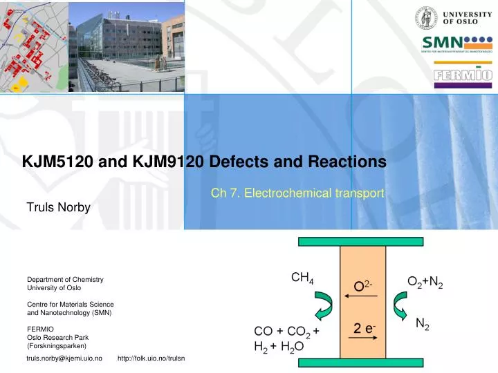
KJM5120 and KJM9120 Defects and Reactions. Ch 7. Electrochemical transport. Truls Norby. Electrochemical transport. Electrochemistry is red-ox-chemistry reduction – uptake of electrons oxidation – loss of electrons

E N D
KJM5120 and KJM9120 Defects and Reactions Ch 7. Electrochemical transport Truls Norby
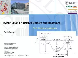
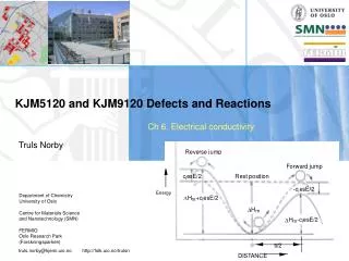
Electrochemical transport • Electrochemistry is red-ox-chemistry • reduction – uptake of electrons • oxidation – loss of electrons • In electrochemistry the reduction and oxidation take place at different locations. • Thus, the overall reaction requires transport of both electrons and of ions (chemical species). • We may expose the material to a gradient in electrical potential, and this will result in a generation of a chemical potential gradient. • Correspondingly, a chemical potential gradient will generate an electrical potential gradient. • We will in this chapter thus treat coexistent chemical and electrical potential gradients and simultaneous transport of at least two charged species. • We will use formalisms and relationships from the two preceding chapters.
Electrochemical potential • A charged species i feels both its own chemical potential and an electrical potential. The combined potential is its electrochemical potential, ηi (”eta”). • The electrochemical potential ηi of a charged species i has a chemical component and an electrical component: • The electrochemical potential gradient in one dimension:
Flux equations (“Wagner theory”) • We shall now derive general equations for the flux and current densities of the species i. • We shall then consider the result of the simultaneous transport of all species by summing up all the current densities into a total (net) current density. • Based on this we shall derive the electrical potential gradient and the voltage over a sample exposed to a chemical potential gradient. • We shall evaluate the case that the net current is zero. • We then derive equations for the flux density of individual species. From this we can evaluate mass transport through the material in several cases of applications. • The procedure is called Wagner theory, after Carl Wagner, who first derived it and used it for analysis of oxidation of metals.
Flux equations (“Wagner theory”) A couple of things to be aware of: • Our procedure (derivation) will be a kind of recipe. • We will do the derivation of Wagner theory first in the general case. • Then we will repeat it for simplified example cases. • We will use real species, not defects. • A reason for this is that electrochemical transport involves exchange of mass and electrons with external phases (e.g. gas phase and electrodes). It is then easier and more consistent to deal with real species. • We insert defects only at the end when we want to evaluate the final expressions – e.g. their pO2 and T dependencies, or their relationship with component or defect diffusivity. …you are kind of expected to learn it…
Flux density of species i • The flux density of any species is ideally given by the concentration, mobility, and the driving force, i.e. the potential gradient: • Via the Nernst-Einstein relations we may choose to express mobility by diffusivity: • or conductivity: Recommendation: Learn one or more of these by heart!
Current density • The current density ii of species i is obtained by multiplying its flux density by its charge:
Total (net) current density • The total (net) current density is obtained by summing over all charge carriers k: • (The reason we choose to call all charge carriers k is that we will return to one of them, i, later on.) • Total, net current must be extracted or supplied through an external circuit. • Typical considerations of total (net) current: • Fuel cell: • At open circuit, there is no net current: itot = 0 • Under load, the net current itot is non-zero. • Mixed ion-electron conducting gas separation membrane: • There are no electrodes or external circuitry; no possibility of net current • Solid-state reaction, e.g. growth of oxide on a corroding metal: • No electrodes or external circuitry; no possibility of net current
Solve for the potential gradient • We now solve the expression for total current density with respect to the electrical potential gradient. Rearrange: Here we use the definitions of total conductivity and transport number
The electrical potential gradient • The expression we obtained This part represents the voltage drop resulting from a current through a material with a certain conductivity (inverse of resistance). It corresponds to Ohm’s law. It is typically Ohmic part Ohmic loss IR-loss This part is the contribution to the potential gradient from gradients in chemical potentials of charge carriers with significant transport numbers tk. It is typically how a fuel cell gets its voltage from a gradient in the chemical potential of oxide ions or protons. Or how a battery gets its potential from a gradient in the activity of e.g. Li+ ions. However, we have a problem: All the species k in the summation are charge carriers, i.e. ions or electrons. This means that their chemical potentials μkare not well-defined, and we will therefore not directly be able to evaluate the expressions. The next thing we need to do is thus to express chemical potentials of charged species by chemical potentials of neutral well-defined species.
Chemical potential gradients of charged vs neutral species • We need to assume and use equilibrium between charged and neutral species. As a general example for species “S”, consider the formation of a charged ion from the neutral atom (where z can be positive or negative). • Equilibrium in this equation along any coordinate is expressed as or, rearranged, • In the x-direction, This expresses the chemical activity gradient for the charged chemical species (ion) by the chemical activity gradient for the neutral atom and for electrons. We will now insert this for the species in the expression for the electrical potential gradient.
Insert for chemical potential of ions • For all ions n (among k) we now insert for the chemical potential gradient. from all ions electrons We have thus obtained an expression containing chemical potentials of neutral atoms, and their ions’ charge and transport numbers. In addition we have a term containing the chemical potential of electrons. This expression contains the essential information of the electrical potential in the sample, and will be used onwards to obtain “everything else” we want to know.
The voltage over a sample • In order to obtain the voltage (potential difference) over a sample, we integrate the potential gradient over the thickness of the sample, from side I to side II: Assume same electrode material on both sides, so that μe,II = μe,I Note ohmic part and chemical potential part, as discussed earlier
The voltage over a sample • In case of open-circuit, itot = 0: • If itot = constant ≠ 0 (steady state current) and σtot = constant: If n counts only one species, and tn can be assumed constant, the equation becomes very simple, and is used for e.g. open circuit voltage of fuel cells and batteries, galvanic sensors, and for determination of transport numbers. We shall return to specific cases later on. Note ohmic (“IR”) part and chemical potential part, as discussed earlier
Flux density of a particular species i • If we wish to know the flux density of one particular species i, we insert the obtained electrical potential gradient (from 2 slides back) into the initial expression of flux density for that species i to obtain
Flux density of a particular species • The flux density of species i in a situation with many species (k): • The flux density is given for a given position with its gradients. The flux of species i from total current and its own transport number The flux of i from its conductivity and own chemical driving force The flux of i from its conductivity and electrical potential driving force controlled by all species
Flux density of a particular species • We now integrate the flux density over the thickness of the sample, from side I to side II.
Flux density - steady-state • We further assume that the flux density of i and total (net) current density are constant through the thickness of the sample: • In this way, we have imposed steady state conditions. • If the transport number ti can be taken as constant, we have or, by dividing throughout by X, X is total thickness from I to II Note that flux is inversely proportional to thickness
Allrighty! • That concludes our first travel through “Wagner-space” for electrochemical transport in solids, using general equations and real species. • The recipe was: • Flux density for each species from diffusivity, mobility, or conductivity, and electrochemical potential gradient. • Current density for each species by multiplication with charge. • Sum all current densities. • Solve for the electrical potential gradient. • Obtain the voltage over the sample by integration, if of interest. • Insert electrical potential gradient back into expression for flux density of individual species. • Flux density obtained by integration over sample thickness assuming individual fluxes and total current are constant (steady state conditions). • Change from chemical potentials of ions to chemical potentials of neutral species by assuming equilibrium in the ionisation of the neutral species.
Specific example;Mixed oxide ion and electron conductor • Two mobile species; oxide ions O2- (z = -2) and electrons e- (z = -1). • Flux densities: • Current densities: • Total current density:
Specific example;Mixed oxide ion and electron conductor • Solve with respect to potential gradient: • Insert equilibrium between oxide ions, electrons, and neutral oxygen. • We choose to use oxygen molecules: • Insertion into expression for potential gradient:
Specific example;Mixed oxide ion and electron conductor • Sum of all transport numbers is unity: • Integrate to obtain the voltage:
Specific example;Mixed oxide ion and electron conductor • Using we obtain • If the transport number is constant, or an average value can be assumed constant, then EN is the Nernst voltage
Specific example;Mixed oxide ion and electron conductor • Practical use; Measurement of transport number by open circuit voltage (OCV, I= 0) in a small gradient in oxygen partial pressure: • Practical use: Galvanic oxygen sensor using the OCV over a pure oxide ion conducting electrolyte (tO2- = 1) vs a reference pO2: • Practical use: Fuel cell using an oxide ion conducting electrolyte (tO2- = 1):
Flux density of oxide ions • Insert potential gradient • into flux density of oxide ions and get • Integrate:
Flux density of oxide ions Flux due to chemical driving force and mixed conductivity Flux due to net current • If the total (net, external) current is zero, we may simplify: Flux inversely proportional to thickness X Alternative representation of mixed conduction
Assume a simple defect model • Assume oxygen deficiency, like in MaOb-y: • Assume electronic conductivity dominates because of higher mobility of electrons than of oxygen vacancies: • Oxygen ion conductivity: σ0 is the oxide ion conductivity at pO2 = 1 bar
Assume a simple defect model • In order to do the integration, we substitute to obtain • The smallest pO2 (at the reducing side) will dominate the parenthesis (because of the negative power) and the highest pO2 (at the oxidising side) may be neglected to a first approximation. For pO2I>>pO2II:
Ambipolar conductivity and diffusivity • The term for mixed conduction that we used in the example case is called ambipolar conductivity, and can be expressed in several ways: • We can correspondingly express the mixed transport as ambipolar diffusivity
Chemical diffusion coefficient in the case of mixed oxygen vacancy and electron transport • We have seen that Fick’s 1st law can be useful, but what is the diffusion coefficient – generally referred to as the chemical diffusion coefficient - that enters? • We will analyse the chemical diffusion coefficient of oxygen in our example material. • In order to approach that, we need to get hold of the concentration gradient of oxygen in the material. We (may) know the concentration gradient of oxygen vacancies, so we write and manipulate:
Chemical diffusion coefficient in the case of mixed oxygen vacancy and electron transport • Insert into flux equation: • Compare with Fick’s 1st law: and obtain:
Chemical diffusion coefficient in the case of mixed oxygen vacancy and electron transport • Use Nernst-Einstein and to obtain • The chemical diffusion coefficient is: • proportional to the self diffusivity of the oxygen defect (here the vacancy), • proportional to the electronic transport number (but which is often unity), • enhanced by the term which for various limiting cases of simplified defect situations takes on values of 1, 3 or 4, and • fully forwards and backwards transformable into defect diffusivities (and in turn self diffusivities) if we know the transport numbers and how defect concentrations vary with pO2.
ηc EN EOCV = EN EN E < EN ηa Surface and electrode kinetics limitations • For electrochemical cells with electrodes and external circuitry, we often express the voltage over the external circuit (load) as consiting of the Nernst voltage minus the IR drop and the electrode overpotentials: or • Membranes without electrodes may have surface kinetics limitations; the effect is the same, but the electrode overpotentials must then be replaced by chemical potential drops
EN EOCV = EN Typical redox reactions Example of individual steps (cathode): Cathode Anode
Interface kinetics – exchange flux and current densities • Equilibrium exchange flux density back and forth across the interface: • where the exchange rate coefficientki is the equivalent of D in bulk diffusion: • Multiply with charge to get exchange current density:
Interface kinetics: Apply a force • A force is applied from a potential step dP, and a net flux over the interface is obtained: • Current density: • If dP = -ηne we obtain the (linear, ohmic, small) overpotential as • Re is called the charge transfer resistance: Note that the interface thickness has dropped out of the expressions and is generally not an essential parameter
Intermezzo • We have made a short analysis of interface processes • r0, ki, j0, i0, and Re were all measures of the random exchange going on at the interface. i0, and Re are the most common to specify. • j, i, and η are the result of force and net flux. They are thus not intrinsic properties of the interface, but proportional to the force. • Next we will couple bulk and interface kinetics
Bulk and surface limitations • Steady state conditions: • The flux through bulk and through surfaces must be the same • Continuity demands that the chemical and electrical potentials match at the interfaces between bulk and surfaces, and that gradients sum up. • But this is difficult to do mathematically and analytically • We resort to chemical diffusion and assume that species flow in concentration gradients both at the surface and in bulk:
Example: Oxygen permeation through a mixed oxide ion and electron conductor; Bulk first • Flux density in bulk: • Introduce ambipolar transport and assume them constant. Integrate: • Rearrange to obtain the chemical potential drop over the bulk:
…then the interface (surface): • Flux given from earlier equatons for interfaces: • and by rearrangement:
The sum of bulk and interface (surface): • The total chemical potential drop is distributed over bulk and interfaces (surfaces): • Insert expressions for the individual potential drops and solve w.r.t. flux: • Critical thickness when surface(s) and bulk contribute equally much: Lcrit = D/k (for one surface) or Lcrit = 2D/k for two surfaces. These expressions are for the case of 2 surfaces Typical critical thickesses: 100 μm Can be affected by surface roughening and catalysts
Back to bulk transport; Anions and cations in a binary oxide MaOb; First some considerations of chemical potential gradients • The formation of the binary oxide • has equilibrium condition: • By inserting and we obtain Since MaOb is present as a pure, condensed phase Important and useful relationship between gradients in the chemical potential of anions and cations. Note the opposite signs!
Anion and cation chemical and electrochemical gradients • From previous slide: • We add on both sides and rearrange to get: • This may be inserted into the total ionic current density to obtain The total ionic current can thus be obtained from a single chemical potential gradient. Note that anions and cations go in opposite directions, but contribute to the same sign of current.
Minority cation diffusion of oxide ion conducting membranes • Cations diffuse towards low chemical potential of metal, i.e. towards high chemical potential of oxygen • This leads to chemical creep (membrane walkout) • If there are more than one cation, different diffusivities may additionally lead to • Demixing • Decomposition (even if the compound is stable per se under both sets of conditions)
La Examples of determination of minor cation diffusion in La2NiO4 • Solid state reaction • Self-diffusion coefficient by diffusion couples • Wagner’s parabolic rate law • In our studies: La2O3+NiO = La2NiO4 yielded DNi • Inter-diffusion • Inter-diffusion coefficient by diffusion couples • Fick’s second law • In our studies: Nd2NiO4 or La2CuO4 vsLa2NiO4 • Tracer diffusion • Tracer-diffusion coefficient by tracer isotope • Radio tracer (radiation count) or chemical tracer (SIMS) • Fick’s second law • In our studies: Chemical tracers Pr and Co From Thesis work of Nebojsa Cebasek, UiO
Metal oxidises and forms a dense oxide layer a M(s) + b/2 O2(g) = MaOb(s) If the oxide forms a dense scale, then the rate of growth dx/dt should be inversely proportional to the scale thickness d: In integrated form: kp = 2kp* and kp* are parabolic rate constants. High temperature oxidation of metals: Wagner oxidation theory
Currents in the oxide scale on a metal • Ionic current has contributions from anions and cations: • Electronic current: • Sum itot = iion + iel = 0 inserted and solve with respect to one current:
From ionic current to scale growth rate • Total ionic current: • Growth rate of MaOb: • Integrate over the scale at steady state:
Parabolic rate constant • From the previous slide: • The term is a form of the parabolic rate constant in the expression • The term σiontel is the ambipolar conductivity. It can be rewritten in many forms, e.g. σeltion. Often the material is either mainly an electronic or an ionic conductor such that a transport number can be set equal to unity. • Often the rate limiting conductivity (ionic or electronic) is dominated by one species (cations or anions). Moreover, often one defect mechanism prevails (vacancies or interstitials, electrons or holes). • In these cases we can integrate the expression analytically if the prevailing defect structure is known or can be anticipated. 3 important paragraphs! More detail in the text.
Example: Growth of Ma-yOb • How did we get here?: • How do we get here?: • Introduce cation vacancies: • Defect chemistry: • Equilibrium constant + electroneutrality gives: and then we are in the position to integrate! This part done differently than in the text