Download

1 / 26
280 likes | 632 Views
Energy. KJM5120 and KJM9120 Defects and Reactions . Ch 6. Electrical conductivity . Truls Norby. Electrical conductivity – before we begin…. In this chapter we will see what happens when we apply an electrical field to mobile charged species.

E N D
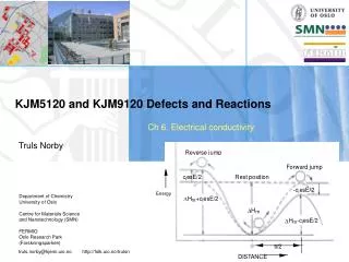
Energy KJM5120 and KJM9120 Defects and Reactions Ch 6. Electrical conductivity Truls Norby
Electrical conductivity – before we begin… • In this chapter we will see what happens when we apply an electrical field to mobile charged species. • From this we will obtain an expression and definition of conductivity. • The conductivity is the proportionality between electrical field and current density (Ohm’s law). • We will see that the factors of conductivity are the charge, concentration and mobility of the charge carriers. • For atoms and ions, the mobility relates directly to the random diffusivity. • For electronic defects, transport may comprise mechanisms different than random diffusion.
Force and flux density in an electrical field • An electrical field (in one dimension) is the downhill gradient in electrical potential: • It gives rise to a force on charged particles given as • We have seen earlier that a force Fi exerted on particles i gives rise to a drift velocity viwhich is proportional to the mechanical mobility Bi: • The flux density after inserting the driving force of the electrical field:
Current density • The current density is the product of charge and flux density:
Charge mobility u is in physics often denoted μ. We here use u to avoid confusion with chemical potential. Very important! Know it! Mobilities and conductivity • We now define a charge mobility ui • We then obtain for the current density: • We now define conductivity σi • and obtain This is a version of Ohm’s law. Conductivity has units S/cm or S/m.
Partial and total conductivity; transport numbers • Total conductivity is the sum of the partial conductivities • The transport number is • Partial conductivities typically comprise cations, anions, electrons, holes: • Each ionic conductivity may have contributions from more than one defect mechanism. • Conductivity from foreign species may contribute, notably protons.
The Nernst-Einstein relation between mobility and diffusion coefficient • We have – from general considerations of transport in a force field - earlier seen that • and, now, through introduction of charge mobility and conductivity: • These are Nernst-Einstein relations. • Now we will derive this in more detail based on random diffusion.
Energy The Nernst-Einstein relation between mobility and diffusion coefficient We will consider an electrical field E superimposed on an energy landscape for randomly jumping charged particles All “ci” in Kofstad’s figure should be “zi” !
Energy The Nernst-Einstein relation between mobility and diffusion coefficient The electrical field E changes the energy barrier in the forward and backward directions. The change depends on the potential difference (distance s x field E) and the charge zie. This changes the rate of forward and reverse sufficiently energetic vibrations
Energy The Nernst-Einstein relation between mobility and diffusion coefficient Flux densities:
The Nernst-Einstein relation between mobility and diffusion coefficient Flux densities: For small ziesE << kT, using ex – e-x≈ 2x for x <<1, we get This is the full non-linear solution for 1-dimensional transport in a material, across an interface, etc. (Butler-Volmer equation) This is the linear (“ohmic”) simplification we get for small fields (i.e. small voltage/distance). It relates net flux density to random diffusivity!
The Nernst-Einstein relation between mobility and diffusion coefficient • From earlier, • Herein lies again the Nernst-Einstein relations: • or, inverted: • The following functions have the same temperature dependence as diffusivity:
Diffusion and mobility • We have considered diffusion and mobility of diffusing species • Applies to atoms and ions in solids, and deeply trapped electrons (and holes (small polarons) • Linear property if driving force not too big • Next we will consider electronic charge carriers • They may travel as free waves (itinerant) and then have drift mobilities, limited by collisions with phonons, impurities, or other defects or be shallowly trapped as large polarons or be deeply trapped as small polarons, whereby they migrate by diffusion
Non-polar solids; itinerant electrons • High temperatures; Mobility dominated by lattice (phonon) scattering. • Typical behaviour: un,latt = un,latt,0 T-3/2 up,latt = up,latt,0 T-3/2 • Low temperatures; Mobility dominated by impurity (defect) scattering. • Typical behaviour: un,latt = un,imp,0 T+3/2 up,latt = up,imp,0 T+3/2 • The total scattering has contributions from both:
Called Eu in the text Polar (ionic) oxides • Large (shallow) polarons Typical behaviour: ularge pol. = ularge pol.,0 T-1/2 • Small (deep) polarons Activated diffusion of electrons or holes: • Note that electrons and holes may migrate by different mechanisms
From mobility to conductivity • Now we have the appropriate expressions of charge mobility • From Chapters 1-4 we have expressions for defect concentrations • From earlier we have • Voila! • But shall we use defects or real species? You can choose – the conductivity is the same - but stick with your choice! • 1st approximation: The concentration of the defect varies, but its mobility is constant The concentration of the constituent ion is constant, but the mobility varies You must under-stand why!
Both NCNV and un+up may contain temperature dependencies, but the exponential Eg/2 dependence often dominates intrinsic semiconductors Intrinsic electronic semiconductors • Electronic conductors: Sum of n-type and p-type contributions: • From Ch. 3; Excitation of electrons and holes: • From Ch. 3; If intrinsic electronic excitation dominates: • Electronic conductivity in intrinsically excited semiconductor:
Temperature dependencies only from mobility Doped semiconductors • At not too low temperatures (kT>>Ed,Ea) effectively all donors and acceptors are ionised • The concentration of electrons or holes is then constant and equal to the donor or acceptor concentration, respectively • Donor-doped semiconductor (n-type): • Acceptor-doped semiconductor (p-type):
Typically, semiconductors have 3 temperature dependency regions • High temperatures • Intrinsic semiconduction (n + p type • Temperature dependency roughly determined by Eg/2 • Intermediate temperatures • n or p determined by donors or acceptors • Temperature dependency given by mobility terms only • Low temperatures • Dopants not effectively ionised • n or p given by ionisation of dopants • Temperature dependency has contributions from Ed or Ea and from mobility un or up
Conductivity in non-stoichiometric oxides • Consider an oxide with oxygen deficiency. From Ch. 3: • The total conductivity may be assumed to be • The mobility of electronic defects (here electrons) is normally orders of magnitude higher than that of point defects (here oxygen vacancies). • so that the conductivity is dominatedly n-type electronic:
pO2 dependency of the n-type conductivity of the oxygen deficient oxide • From previous slide: • Let’s take the logarithm: • Log conductivity vs log pO2 gives a straight line with slope -1/6 • An observed dependency like this would be characteristic for and thus used to identify the simplified electroneutrality at hand • Note the isobar (at constant pO2) for the next slide
Temperature dependency of the n-type conductivity of the oxygen deficient oxide • From previous slide: • Let us assume a small polaron hopping model for electrons: • Let’s take the logarithm: • An isobaric plot of log(σnT) vs 1/T (Arrhenius plot) yields the activation energy. which has contributions from defect formation and mobility
Ionic conductivity; Example: Y-doped ZrO2 • If we acceptor dope ZrO2-y with Y2O3 (yttria stabilised zrconia, YSZ) we get • and the ionic conductivity due to oxygen vacancies becomes • This conductivity is independent of pO2 • A plot of ln(σvO**T) vs 1/T yields the activation energy for mobility of oxygen vacancies from the slope
Three (or four) regions of temperature dependency for a doped ionic conductor • High temperatures • Intrinsic defect pair or non-stoichiometry dominate • Normally electronic conduction • Moderately high temperatures • Dopant and ionic defect dominate • But electronic defects significant, and their mobilities make them dominate conductivity • Moderately low temperatures • Dopant and ionic defect dominate • High ionic conductivity • Temperature dependency reflects activation energy of mobility of ionic defect • Low temperatures • Mobile defects trapped by dopants • Low ionic conductivity • Temperature dependency reflects both mobility of the defect and the trapping energy
From concentration properly to conductivity • The concentration in conductivity expressions must be a volume concentration: • #/unit volume (e.g. cm-3 or m-3) or (if e is replaced by F) • mol/unit volume (e.g. mol cm-3) • Thus, if the concentration is originally obtained from defect chemistry as site fraction or molar fraction, it must be converted to volume concentration by multiplying with the site density or molar density; generally: • Examples: • Site density cs obtained from number of sites per formula unit b times Z (number of formula units per unit cell) divided by unit cell volume Vu: cs = b * Z / Vu • Molar density obtained as mass density δ divided by molar mass Mm: Cm (mol/unit volume) = δ (mass/unit volume) / Mm (mass/mol) • Molar density is the inverse of molar volume Vm: Cm = 1 / Vm
Correlation factor • The effective diffusion of a traceable ion (tracer) is not necessarily as large as that of a non-traceable one (or of charge itself): Dt = f Dr where f≤ 1 (depending on structure and diffusion mechanism) so that Dt ≤ Dr. • In intersticialcy diffusion, we have the additional action of a displacement factor S; ratio between charge displacement and tracer displacement: Dt = (f/S) Dr • f and S can be evaluated from ionic conductivity and Dt (Individual measurements or the Manning experiment) S = 2