Download

1 / 42
440 likes | 830 Views
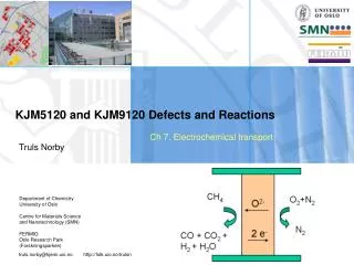
KJM5120 and KJM9120 Defects and Reactions . Ch 5. Diffusion . Truls Norby. Diffusion – important property!. Diffusion describes transport of species (particles, atoms, ions, molecules) through a medium (gas, liquid, solid) Here we consider only solid-state diffusion

E N D
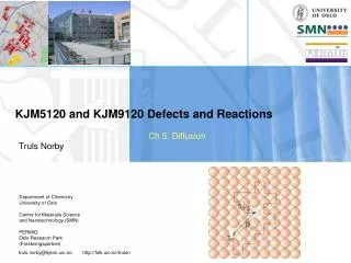
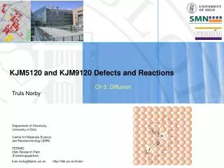
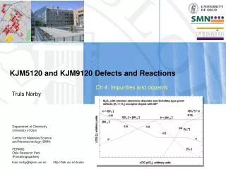
KJM5120 and KJM9120 Defects and Reactions Ch 5. Diffusion Truls Norby
Diffusion – important property! • Diffusion describes transport of species (particles, atoms, ions, molecules) through a medium (gas, liquid, solid) • Here we consider only solid-state diffusion • Diffusion in crystalline solids takes place only by defects; in a perfect structure, there can be no diffusion • Many essential processes take place by solid-state diffusion: Reactions, synthesis, mixing, doping, permeation, ionic conduction, sintering, grain growth, creep, corrosion, a.o. • These comprise the synthesis, fabrication, utilisation, and breakdown of materials
Don’t worry (yet)! These are the things we’ll learn to sort out in this chapter and in Ch. 7 Diffusion – many terms • There are many terms of diffusion • Random diffusion • Self diffusion • Defect diffusion • Tracer diffusion • Chemical diffusion • Ambipolar diffusion • Random diffusion is caused only by thermal energy and does not require any gradients or driving force • Self diffusion reflects random diffusion of a component (e.g. oxide ions) • Defect diffusion reflects random diffusion of a defect • The remaining terms reflect diffusion with a net transport in some direction, driven by a gradient – a driving force • However, also these gradient-driven diffusion phenomena are governed by random, thermally activated diffusion!
Diffusion - knowing defects brings insight • Diffusion is considered a difficult theme, because of the many terms and how they are interlinked. • The difficulties arise especially in the presence of driving forces. • Diffusion coefficients in driving forces are often termed chemical diffusion coefficients, and without understanding of defects, they may remain obscure and phenomenological. • However, by understanding defects, it is possible to get control of it all. This is actually one of the main goals of the course. • In this Ch 5. we mostly deal with random, thermally driven diffusion. • In Ch. 6 we deal with diffusion of charged species under an electrical field, i.e. electrical conduction. • In Ch. 7 we deal with the combination of electrical and chemical driving forces – electrochemical transport.
Diffusion – our approach • Diffusion not only has many terms, it is also somewhat abstract… …the physical meaning of the property diffusivity may be and may remain difficult to grasp… we will therefore try to see it and express it in terms of more physical terms. • We will approach diffusion by introducing you to several models - pictures and relationships - of diffusion. They will give various examples of what diffusion is. They may seem different and inconsistent...don’t let this disencourage you.
Before we really start…. • …let us have a look at another type of diffusion; thermal diffusion • Fourier found that the flux of heat through a medium is proportional to the temperature gradient. In one dimension this is written: • The proportionality coefficient κ (kappa) is termed the thermal conductivity. (A better term might be thermal diffusivity?) It has units of J/(cm s K). • Note that the temperature gradient is positive in the direction of increasing temperature (uphill). • The minus sign in the equation thus tells us that the heat flows downhill – from high to low temperature. Fourier’s law of heat flux. jq is a flux density and has units of e.g. J/(cm2s)
Fick’s first law of diffusion • Fick proposed a relationship of diffusion of matter similar to Fourier’s equation for heat. He proposed that the flux of particles is proportional to the gradient in concentration of particles. In one dimension this is written: • The flux density j of particles has units e.g. #/(cm2s) or mol/(cm2s) • The concentration is given in e.g. #/cm3 or mol/cm3 • The diffusion coefficient (or diffusion constant) then has units cm2/s • The minus sign states that the flux goes down the concentration gradient. The negative of the concentration gradient may be taken as the driving force.
Fick’s first law of diffusion - comments • Fick’s first law is a phenomenological – or empirical – expression; It describes a flux in terms of a concentration gradient and a proportionality coefficient – the diffusion coefficient, or diffusivity. • However, Fick’s first law applies strictly only to neutral non-interacting particles. Examples comprise dilute solutions of interstitial atoms, e.g. atomic H in metals. • For other situations, the coefficient in Fick’s first law is not a constant. • D in Fick’s first law has not been given any physical meaning upto now – it remains a phenomenological coefficient. In the next model, we will give it more content.
Potential gradient as the driving force • Consider particles (or a species) i and that it feels a force Fi in some direction. • The flux density of i (flux of particles i through a plane of unit area per unit time) is given by the concentration of particles i and the average net drift velocity of particles i: • The drift velocity is proportional to the driving force: • The proportionality between force and velocity is the mechanical mobility B (“beweglichkeit”). It says something about how easy it is to move something, like the inverse of friction.
The force is a field: Potential gradient • The force Fi is a field; the negative (downhill) gradient in a potential Pi. In one dimension; • Insertion gives • We see that the flux density is given by the concentration, the mobility, and the driving force (negative of potential gradient), which all make sense.
This series is important. Be sure you understand all parts. The last one uses dlnc = 1/c. Example: Chemical potential gradient acting on neutral particles • Consider a neutral species i experiencing a chemical potentialμi: • The driving force, potential gradient is then • Insert into the flux density expression: • By comparison with Fick’s first law, we see that • In other words; For neutral non-interacting particles, Fick’s first law is valid (D is independent of concentration). • D is the product of mechanical mobility B and thermal energy kT.
Brief recap; Diffusivity and mobility • We have by now seen diffusion as a macroscopic process wherein matter flows from a region of high to a region of low concentration, down a concentration gradient. • We have seen that a more accurate and physical example of this is the flow in a chemical potential gradient. • This has enabled us to see that the diffusion coefficient D is the product of mechanical mobility B (“beweglichkeit”) and thermal energy kT. From this we may conclude that diffusivity is driven by thermal energy and that the mobility tells how easily it is driven. • D = kTB is in fact a definition of D. It is one form of the Nernst-Einstein relation. • For neutral non-interacting particles, the diffusivity D = kTB enters Fick’s first law.
Microscopic model – one-dimensional diffusion • Consider a solid, divided into parallel planes normal to the x direction. The distance between planes equals the jump distance s for particles. • The number of particles per unit area of a plane p is termed np. • Consider jumps in the x direction: Particles jump at rate Γ (gamma) from one plane into one of the two neighbouring planes. • The rate of particles jumping from a plane p into a neighbouring plane, per unit area, is thus ½npΓ. • The net flux from plane 1 to plane 2 is thus the difference between the flux from 1 to 2 and the flux from 2 to 1:
….introduce volume concentration and concentration gradient… • The number of particles in unit area of the plane p is given by the volume concentration cp and the thickness of the planes (i.e. the plane distance): • Insertion into the flux yields • The difference in concentrations between planes can be expressed in terms of a concentration gradient, e.g. • Insert into flux expression
…and in 3 dimensions… • In the case of 1-dimensional diffusion, ½ of the particle’s jumps took place in the forward x direction. • If the particles can jump orthogonally in 3 dimensions, only 1/6 of the jumps take place in the forward x direction. We would then obtain • From comparison with Fick’s first law, we now see that the diffusion coefficient D is given by 1/6 the jump rate times the jump length squared:
How fast and how far? • The jump rate Γ can be expressed in terms of the number of jumps n per time t: • Rearranging, we get: • Interstitial diffusion of oxygen atoms in niobium metal at 800 °C; • D = 7·10-8 cm2s-1. • The jump distance s = 1.65 Å (1.65·10-8 cm). • Then the jump frequency Γ is about 1.54·109 s-1. • In 1 second the atom travels 25 cm! In one hour it travels almost 1 km! • But the travel is random…statistically it gets nowhere! Total travelled distance in time t Total number of jumps in time t
Brief recap: Net diffusion in a gradient and random diffusion suddenly merged?? • Yes! • Net flow due to diffusion in a gradient is in fact random diffusion, just with a small statistically increased chance of random jumps from larger to smaller concentration, just because there are more atoms to jump from high concentration than from low concentration. • Therefore we have been able to link net diffusion in a gradient mathematically to the random diffusion coefficient. • And vice versa, we have perhaps gotten a more “humane” picture of random diffusion, by taking it as part of a “normal” diffusion flow process. • Next, we shall look in more detail at the randomness of random diffusion.
Root mean square displacement…the mean distance a particle travels from the starting point Random diffusion • Total displacement is the sum of all individual jumps: • Take square to obtain length: • Rightmost term approaches zero as number of jumps becomes very large. Leftmost term represents the mean squared displacement:
Random diffusion • Statistically summed over all directions • 2 in 1-dimensional diffusion • 4 in 2-dimensional diffusion • 6 in 3-dimensional diffusion the particle gets nowhere; it most likely ends where it started. • Still, the mean distance has a non-zero value. • The root mean square displacement represents an effective diffusion length away from the starting point when averaged over all particles after a large number of jumps. • The RMS displacement represents the radius of a sphere around the starting point in 3-dimensional diffusion.
_ Rn Random 3-dimensional diffusion; displacement in one direction • The RMS displacement represents the radius of a sphere around the starting point in 3-dimensional diffusion. • If we, however, are interested in diffusion only in one direction, the effective length is smaller. This may be seen as a consequence of 2/3 of the jumps represented by the diffusion coefficient being ineffective for our interest; • This length is for instance a best estimate of the effective diffusion length of a species into a specimen starting at the surface. The diffusion process is 3-dimensional, but we measure the penetration length only in one dimension. x
Brief recap; Random diffusion • This has ended our tour of models of random diffusion • Random diffusion is really …..random! Species diffuse….they travel far, but get very short. • When we expose a system to a gradient in concentration, we may get a net flux…but it is merely a perturbation of the random diffusion. • Oxygen diffusion in niobium: The oxygen atoms on average jump 1.54·109 times per second at 800 °C. From these considerations we estimated that an oxygen atom has randomly covered total jump distances of 915 m in 1 hour. • But what is the mean displacement? One may estimate that the one-dimensional root-mean-square displacement after 1 hour amounts only to 0.022 cm! • Thus, the oxygen atoms spend most of their time jumping "back and forth".
1 2 Fick’s second law of diffusion - concept • Before we go deeper into diffusion mechanisms, we stop by an important use of the simple phenomenological diffusion coefficients that appeared in Fick’s first law. • Fick’s first law assumes a fixed concentration gradient. • In many cases the gradient changes with position x and consequently also with time.
1 2 Fick’s second law of diffusion – qualitative approach • Consider the two planes 1 and 2 in the figure. • The gradient in 1 is larger than in 2. According to Ficks’s first law the net flux to the right is thus larger in 1 than in 2. • The middle figure shows that the flux varies with x. The slope is dj/dx. • Right-hand side figure: The flux j1 into the region between the two planes is thus higher than the flux j2 out of the region. • Thus the concentration in the “concave” region between 1 and 2 increases, seeking to even out the differences in gradient and flux. • Correspondingly a region with a “convex” concentration curve would decrease in concentration, also to even out the differences.
1 2 Fick’s second law of diffusion - mathematics • It may be shown that the change in concentration is given by the gradient in flux density: • Fick’s first law applies in each point along x, and we may thus insert for the flux density j so as to get: • If D is independent of c, we may simplify: • Especially the last equation may be solved for many practically achievable geometries and boundary conditions. These are different versions of Fick’s second law of diffusion The “bible” of solutions to Fick’s second law is J. Crank (1956); “Mathematics of diffusion”
Example of use of Fick’s 2nd law • Tracer diffusion into a solid from a finite source at the surface • Procedure: • Polish the surface. • Apply a thin film source of a chemical or isotope tracer on the surface. • Anneal the sample at elevated temperature for a given time t. • Analyse the depth profile of the tracer concentration vs depth x. • Sectioning/radiography • SIMS • The appropriate solution to Fick’s 2nd law is • where c0 is the starting concentration of the tracer at the surface (x=0) at t=0. Tracer diffusion coefficient obtained from slope in plot of lnc vs x2. At the point where c(x) = c0/2 we have x = (2.77Dtt)1/2. This corresponds approximately to the root-mean-square penetration distance x = (2.77Dtt)1/2.
Example of use of Fick’s 2nd law • Tracer diffusion into a solid from a constant (infinite) source at the surface • Procedure: • Polish the surface. • Apply a chemical or isotope tracer on the surface in a separate phase (gas, liquid, solid) with constant activity of the tracer. • Anneal the sample at elevated temperature for a given time t. • Analyse the depth profile of the tracer concentration vs depth x. • Sectioning/radiography • SIMS • The appropriate solution to Fick’s 2nd law is • where c0 is the background concentration of the tracer in the solid and cs is the constant source concentration. erf is the so-called error function. Find Dt by numerical fitting. Profile under assumption that c0 = 0.
Diffusion coefficients • We have seen two examples of how tracer diffusion coefficients that enter as constant in Fick’s 2nd law can be determined. • In Ch. 6 we will see how ionic conductivity is directly proportional to the random diffusion coefficient of the ion and can be used to determine the latter. • In Ch. 7 we will see how various more complex processes (reactions, interdiffusion, corrosion, permeation, creep, etc.) are related to diffusion coefficients and can be used to determine them. • Now, we will first look at the actual microscopic mechanisms of diffusion via defects.
Diffusion mechanisms • Two important mechanisms: Vacancy mechanism • Predominant for native atoms and ions Interstitial mechanism • Predominant for small interstitially dissolved foreign atoms and ions • Significant for native atoms and ions only in relatively open structures
Diffusion mechanisms • More special mechanisms: • Interstitialcy mechanisms • Collinear • Non-collinear • Crowdion • Simultaneous movement of many atoms • Ring mechanisms
Diffusion mechanisms • Diffusion of protons in oxides • Free proton jumps from oxide ion to oxide ion (Grotthuss mechanism) • H+ • Vehicle mechanisms (not important in crystalline solids) • OH- • H2O • H3O+ • NH2- • NH4+
Factors that affect diffusivity • We have seen that the random diffusion coefficient can be expressed in terms of jump distance s and jump rate Γ(number of jumps n per time t): • We shall now analyse the jump rate in more detail. • It contains a number of factors: • The vibration frequency • The ratio of vibrations sufficiently energetic to make the jump • The number of neighbouring sites to jump to • The chance (ratio) that the jumping particle is free to jump. • The chance (ratio) that the site jumped to can receive it. Attempt frequency Defect concentration enters here when applicable
a0 Diffusion by vacancy mechanism • Jump rate is proportional to the attempt frequency, number of neighbouring sites to jump to, and the concentration (fraction) of vacancies (defects) • The diffusivity thus becomes • Example: bcc structure: Z = 8, s = √3 a0/2. • In general, we collect all geometrical factors in a parameter α: (For bcc and fcc, α = 1)
Diffusion by interstitial mechanism • Diffusion of an interstitially dissolved foreign atom • The chance that the atom is interstitial is unity. • The chance that the neighbouring (interstitial) position is vacant is close to unity when the concentration of interstitials is small. • Diffusion of a component species by interstitial mechanism • In this case, the chance that a component atom is interstitial, Nd, enters. Thus, for component species, the defect concentration enters either way!
How does D vary with T and pO2? • We start by analysing the influence from the concentration of defects. • Example:Vacancies in an elemental solid: • Example: Oxide ion vacancies in a non-stoichiometric oxide, e.g. MaOb-δ: • Example: Oxide ion vacancies in an acceptor-doped oxide, e.g. Ca-doped ZrO2-δ:
Important equation Temperature dependency of ω • The rate of sufficiently energetic vibrations contains • vibration frequency ν (”nu”) • Gibbs energy of the activated saddle point complex • Activation entropy • Activation enthalpy • It is common to disregard the entropy and consider the enthalpy as dominating for Gibbs energy. • It is common to find that the vibration frequency increases with increasing barrier height: • This gives a ”compensation” effect often referred to as a Meyer-Neldel effect. ,
Example of full expression: Vacancy diffusion in an elemental solid • The general expression for random (self) diffusion: • The expression for the fraction of defects: • The expression for the rate of sufficiently energetic jump attempts: • The final, full, expression: Temperature-independent part D0 Temperature-dependent part; activation energy Q contains enthalpy of defect formation plus enthalpy of jump activation
Example of full expression: Vacancy diffusion in an elemental solid; concentration “frozen in” • The general expression for random (self) diffusion: • The expression for the fraction of defects: • The expression for the rate of sufficiently energetic jump attempts: • The final, full, expression: Temperature-independent part D0 Temperature-dependent part; activation energy Q contains enthalpy of jump activation only
Example of full expression: Vacancy diffusion in an oxygen deficient oxide • The general expression for random (self) diffusion: • The expression for the fraction of defects: • The expression for the rate of sufficiently energetic jump attempts: • The final, full, expression: pO2 dependency Temperature-dependent part; activation energy Q contains enthalpy of defect formation divided by 3 (the number of defects formed), plus enthalpy of jump activation Temperature-independent part D0
Example of full expression: Vacancy diffusion in an acceptor-doped oxide • The general expression for random (self) diffusion: • The expression for the fraction of defects, e.g.: • The expression for the rate of sufficiently energetic jump attempts: • The final, full, expression: (No pO2 dependency) Temperature-dependent part; activation energy Q contains enthalpy of jump activation only Temperature-independent part D0
Diffusion coefficients of point defects • We now consider the diffusion of the point defect itself instead of the constituent (structural) species. • A vacancy needs to hit an occupied position in order to make a successful jump. Thus, its diffusivity is where N is the fraction of occupied sites (N = 1 – Nd, normally N~ 1) . • Thus, comparison between self-diffusion Dr and vacancy diffusion Dv shows that it follows the general relationship • In other words, the defect diffusion is much faster than the self-diffusion, given by the ratio of defects to normally occupied sites. Important !
Proton diffusion in oxides; isotope effects • Relies on O2- sublattice dynamics Hm,H+ 2/3 Hm,O • ”Simple” H/D/T isotope effects expected: • Classical effect: Vibrations given by reduced mass of O-H oscillator, i.e., close to the 1:2:3 • D0,H:D0,D:D0,T 1/1 : 1/2 : 1/ 3 • Non-classical “zero-level” effect; ΔHm,D–ΔHm,H≤ 0.06 eV. • However, pre-exponentials of proton diffusion typically 10% of classically predicted. • Pre-exponential may be dominated by O-O vibration (=0.1 that of O-H) • Sticking probability for H+ smaller than for D+, and typically 0.1. Counteracts classical effect.
Review • Review the different terms of diffusion – try to recall typical features of their mathematical expressions: • Random diffusion • This is the general term • Self diffusion • For constituents • Defect diffusion • For defects • Tracer diffusion • Equal to or slightly lower than random diffusion • Chemical diffusion • The diffusion coefficient (phenomenological) that enters Fick’s 1st law • Ambipolar diffusion • When two species diffuse dependent of each other – typically ions and electrons. This we will learn in Ch. 7