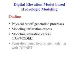
Digital Elevation Model based Hydrologic Modeling
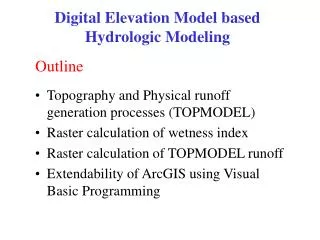
Digital Elevation Model based Hydrologic Modeling. Outline. Topography and Physical runoff generation processes (TOPMODEL) Raster calculation of wetness index Raster calculation of TOPMODEL runoff Extendability of ArcGIS using Visual Basic Programming.

Digital Elevation Model based Hydrologic Modeling
E N D
Presentation Transcript
Digital Elevation Model based Hydrologic Modeling Outline • Topography and Physical runoff generation processes (TOPMODEL) • Raster calculation of wetness index • Raster calculation of TOPMODEL runoff • Extendability of ArcGIS using Visual Basic Programming
Physical Processes involved in Runoff Generation From http://snobear.colorado.edu/IntroHydro/geog_hydro.html
Runoff generation processes P Infiltration excess overland flow aka Horton overland flow f P qo P f Partial area infiltration excess overland flow P P qo P f P Saturation excess overland flow P qo P qr qs
Map of saturated areas showing expansion during a single rainstorm. The solid black shows the saturated area at the beginning of the rain; the lightly shaded area is saturated by the end of the storm and is the area over which the water table had risen to the ground surface. [from Dunne and Leopold, 1978] Seasonal variation in pre-storm saturated area [from Dunne and Leopold, 1978]
Runoff generation at a point depends on • Rainfall intensity or amount • Antecedent conditions • Soils and vegetation • Depth to water table (topography) • Time scale of interest These vary spatially which suggests a spatial geographic approach to runoff estimation
TOPMODEL Beven, K., R. Lamb, P. Quinn, R. Romanowicz and J. Freer, (1995), "TOPMODEL," Chapter 18 in Computer Models of Watershed Hydrology, Edited by V. P. Singh, Water Resources Publications, Highlands Ranch, Colorado, p.627-668. “TOPMODEL is not a hydrological modeling package. It is rather a set of conceptual tools that can be used to reproduce the hydrological behaviour of catchments in a distributed or semi-distributed way, in particular the dynamics of surface or subsurface contributing areas.”
TOPMODEL and GIS • Surface saturation and soil moisture deficits based on topography • Slope • Specific Catchment Area • Topographic Convergence • Partial contributing area concept • Saturation from below (Dunne) runoff generation mechanism
Specific catchment area a is the upslope area per unit contour length [m2/m m] Stream line Contour line Upslope contributing area a Numerical Evaluation with the D Algorithm Topographic Definition Tarboton, D. G., (1997), "A New Method for the Determination of Flow Directions and Contributing Areas in Grid Digital Elevation Models," Water Resources Research, 33(2): 309-319.) (http://www.engineering.usu.edu/cee/faculty/dtarb/dinf.pdf)
Hydrological processes within a catchment are complex, involving: • Macropores • Heterogeneity • Fingering flow • Local pockets of saturation The general tendency of water to flow downhill is however subject to macroscale conceptualization
TOPMODEL assumptions • The dynamics of the saturated zone can be approximated by successive steady state representations. • The hydraulic gradient of the saturated zone can be approximated by the local surface topographic slope, tan. • The distribution of downslope transmissivity with depth is an exponential function of storage deficit or depth to the water table • To is lateral transmissivity [m2/h] • S is local storage deficit [m] • z is local water table depth [m] (=S/ne) • ne is effective porosity • m is a storage-discharge sensitivity parameter [m] • f =ne/m is an alternative storage-discharge sensitivity parameter [m-1]
D Dw S Topmodel - Assumptions • The soil profile at each point has a finite capacity to transport water laterally downslope. e.g. or
D Dw S Topmodel - Assumptions Specific catchment areaa [m2/m m] (per unit contour length) • The actual lateral discharge is proportional to specific catchment area. • R is • Proportionality constant • may be interpreted as “steady state” recharge rate, or “steady state” per unit area contribution to baseflow.
D Dw S Topmodel - Assumptions Specific catchment areaa [m2/m m] (per unit coutour length) • Relative wetness at a point and depth to water table is determined by comparing qact and qcap • Saturation when w > 1. i.e.
D Dw S Topmodel Specific catchment areaa [m2/m m] (per unit coutour length) z
Slope Specific Catchment Area Wetness Index ln(a/S) from Raster Calculator. Average, l = 6.91
Numerical Example • Compute • R=0.0002 m/h • l=6.90 • T=2 m2/hr Given • Ko=10 m/hr • f=5 m-1 • Qb = 0.8 m3/s • A (from GIS) • ne = 0.2 Raster calculator -( [ln(sca/S)] - 6.90)/5+0.46
Calculating Runoff from 25 mm Rainstorm • Flat area’s and z <= 0 • Area fraction (81 + 1246)/15893=8.3% • All rainfall ( 25 mm) is runoff • 0 < z rainfall/effective porosity = 0.025/0.2 = 0.125 m • Area fraction 546/15893 = 3.4% • Runoff is P-z*0.2 • (1 / [Sat_during_rain ]) * (0.025 - (0.2 * [z])) • Mean runoff 0.0113 m =11.3 mm • z > 0.125 m • Area fraction 14020/15893 = 88.2 % • All rainfall infiltrates • Area Average runoff • 11.3 * 0.025 + 25 * 0.083 = 2.47 mm • Volume = 0.00247 * 15893 * 30 * 30 = 35410 m3
GIS estimation of hydrologic response function • Amount of runoff generated • Travel time to outlet • Distance from each grid cell to outlet along flow path (write program to do this) • Distance from each point on contributing area • overlay grid to outlet distances with contributing area.
Steps for distance to outlet program • Read the outlet coordinates • Read the DEM flow direction grid. This is a set of integer values 1 to 8 indicating flow direction • Initialize a distance to outlet grid with a no data value • Convert outlet to row and column references • Start from the outlet point. Set the distance to 0. • Examine each neighboring grid cell and if it drains to the current cell set its distance to the outlet as the distance from it to the current cell plus the distance from the current cell to the outlet.
4 3 2 5 1 6 7 8 Direction encoding 1 2 3 1 7 6 5 2 7 6 5 3 6 7 7 Distances to outlet Programming the calculation of distance to the outlet 102.4 72.4 30 72.4 42.4 0
Visual Basic Programming in ArcMAP References ESRI, (1999), ArcObjects Developers Guide: ArcInfo 8, ESRI Press, Redlands, California. Zeiler, M., (2001), Exploring ArcObjects. Vol 1. Applications and Cartography. Vol 2. Geographic Data Management, ESRI, Redlands, CA.
AREA 2 3 AREA 1 12 Are there any questions ?