Download
1 / 25
250 likes | 341 Views
The Luminosity Calorimeter. Iftach Sadeh Tel Aviv University Desy ( On behalf of the FCAL collaboration ). June 11 th 2008. Overview. 2. Intrinsic properties of LumiCal: Luminosity measurement. Design of LumiCal. Performance of LumiCal. Event reconstruction: Bhabha scattering.

E N D
The Luminosity Calorimeter Iftach SadehTel Aviv UniversityDesy( On behalf of the FCAL collaboration ) June 11th 2008
Overview 2 • Intrinsic properties of LumiCal: • Luminosity measurement. • Design of LumiCal. • Performance of LumiCal. • Event reconstruction: • Bhabha scattering. • Clustering in LumiCal - Algorithm design and performance.
Performance requirements Compare angles & energy X,Y RIGHT θ Z 3 • Required precision is: • Measure luminosity by counting the number of Bhabha events (NB):
Design parameters 4 • 1. Placement: • 2270 mm from the IP • Inner Radius - 80 mm • Outer Radius - 190 mm 2. Segmentation: • 48 azimuthal & 64 radial divisions: • Azimuthal Cell Size - 131 mrad • Radial Cell Size - 0.8 mrad 3. Layers: • Number of layers - 30 • Tungsten Thickness - 3.5 mm • Silicon Thickness - 0.3 mm • Elec. Space - 0.1 mm • Support Thickness - 0.6 mm
ares Intrinsic parameters σ(θ) • Position reconstruction (polar angle): 5 • Relative energy resolution: Bias Logarithmic constant Resolution
Detector signal σ(θ) ares 6 • Distribution of the deposited energy spectrum of a MIP (using 250 GeV muons):MPV of distribution = 89 keV ~ 3.9 fC. • Distributions of the charge in a single cell for 250 GeV electron showers. • The influence of digitization on the energy resolution and on the polar bias. MIPs Digitization Signal distribution
LumiCal Performance antiDID DID 6cm 8cm 19cm 7 • Beamstrahlung spectrum on the face of LumiCal (14 mrad crossing angle): For the antiDID case Rmin must be larger than 7cm.
Beam-Beam effects at the ILC 8 High beam-beam field (~kT) results in energy loss in the form of synchrotron radiation (beamstrahlung). Bunches are deformed by electromagnetic attraction: each beam acting as a focusing lens on the other. Change in the final state polar angle due to deflection by the opposite bunch, as a function of the production polar angle. • Since the beamstrahlung emissions occur asymmetrically between e+ and e-, the acolinearity is increased resulting in a bias in the counting rate. “Impact of beam-beam effects on precision luminosity measurements at the ILC” – C. Rimbaultet al. (http://www.iop.org/EJ/abstract/1748-0221/2/09/P09001/)
Clustering - Detector simulation 9 • 1. Placement: • 2270 mm from the IP • Inner Radius - 80 mm • Outer Radius - 350 mm 2. Segmentation: • 96 azimuthal & 104 radial divisions: • Azimuthal Cell Size - 65.5 mrad • Radial Cell Size - 1.1 mrad • The clustering algorithm was tested for the previous versionof LumiCal: • Larger radius. • Smaller azimuthal cell size. • Larger radial cell size. 3. Layers: • Number of layers - 30 • Tungsten Thickness - 3.5 mm • Silicon Thickness - 0.3 mm • Elec. Space - 0.1 mm • Support Thickness - 0.6 mm
Topology of Bhabha scattering 10 • (3∙104 events of) Bhabha scattering with √s = 500 GeV θ Φ Energy • Separation between photons and leptons, as a function of the energy of the low-energy particle. • Shower profile in LumiCal - The Moliere radius is indicated by the red circle.
Clustering - Algorithm 11 • Longitudinal shower shape. • Phase I:Near-neighbor clustering in a single layer. • Phase II:Cluster-merging in a single layer.
Clustering - Algorithm 12 • Phase III:Global-clustering.
Clustering - Results 13 • (2→1): Two showers were merged into one cluster. • (1→2): One shower was split into two clusters. • The Moliere radius is RM (= 14mm), dpair is the distance between a pair of showers, and Elow is the energy of the low-energy shower.
Clustering - Results (event-by-event) 14 (EGen- ERec)/ EGen • Event-by-event comparison of the energy and position of showers (GEN) and clusters (REC) as a function ofEGen. (ΦGen- ΦRec)/ ΦGen (θGen- θRec)/ θGen
Clustering - Geometry dependence 15 96 div 48 div 24 div
Summary 16 • Intrinsic properties of LumiCal: • Energy resolution: ares ≈ 0.21 √GeV. • Relative error in the luminosity measurement:ΔL/L = 1.5 · 10-4 4 · 10-5 (at 500 fb-1), where the theoretical uncertainty is expected to be ~ 2 · 10-4 . • Event reconstruction (photon counting): • Merging-cuts need to be made on the minimal energy of a cluster and on the separation between any pair of clusters. • The algorithm performs with high efficiency and purity for both the previous and the new design of LumiCal. • The number of radiative photons within a well defined phase-space may be counted with an acceptable uncertainty.
Selection of Bhabha events Simulation distribution Distribution after acceptance and energy balance selection Left side signal Compare angles & energy X,Y RIGHT θ Z Right side signal 18 Acoplanarity Acolinearity Energy Balance
Physics Background leptonic Four-fermion processes hadronic 19 • Four-fermion processes are the main background, dominated by two-photon events (bottom right diagram). BEFORE AFTER cut The cuts reduce the background to the level of 10-4
Digitization ares σ(θ) Δθ
Thickness of the tungsten layers (dlayer) 21 ares Signal distribution Δθ σ(θ)
Effective layer-radius, reff(l) & Moliere Radius, RM 22 • Dependence of the layer-radius, r(l), on the layer number, l. • Distribution of the Moliere radius, RM. r(l) RM
Clustering - Energy density corrections 23 • Event-by-event comparison of the energy of showers (GEN) and clusters (REC). Before After
Clustering - Results (measurable distributions) 24 • Merging-cuts:Elow ≥ 20 GeV , dpair ≥ RM Energylow Energyhigh θhigh θlow Δθhigh,low • Energy and polar angle (θ) of high and low-energy clusters/showers. • Difference in θ between the high and low-energy clusters/showers.
Clustering - Results (relative errors) 25 • Dependence on the merging-cuts of the errors in counting the number of single showers which were reconstructed as two clusters (N1→2), and the number of showers pairs which were reconstructed as single clusters, (N2→1).