Download
1 / 35
350 likes | 372 Views
This workshop presentation discusses the interdecadal variation of the Arctic Oscillation (AO) in historical climate change simulations using a coupled GCM and an atmospheric GCM. The simulations reproduce the observed trend and interdecadal change of the AO, and the results suggest a potential interaction between internal variability and external forcing.

E N D
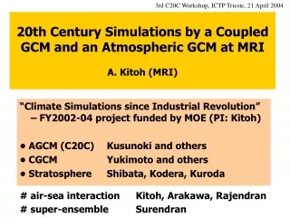
3rd C20C Workshop, ICTP Trieste, 21 April 2004 20th Century Simulations by a Coupled GCM and an Atmospheric GCM at MRIA. Kitoh (MRI) “Climate Simulations since Industrial Revolution” – FY2002-04 project funded by MOE (PI: Kitoh) • AGCM (C20C) Kusunoki and others • CGCM Yukimoto and others • Stratosphere Shibata, Kodera, Kuroda # air-sea interaction Kitoh, Arakawa, Rajendran # super-ensemble Surendran
Interdecadal Variation of the Arctic Oscillation in a Historical Climate Change Simulation with the MRI-CGCM2S. Yukimoto and K. Kodera (MRI) • Simulation of the 20th century climate (CMIP 20C3M) - observed trend - interdecadal variation • Observed climate change and variation in the 20th century - internal variability? - response to external forcing? • Model validation
Observed Arctic Oscillation (AO) ? ? • Interdecadal variation • Negative trend until 1960s • Positive trend afterwards • Internal variability? interaction with the ocean? • Response to external forcing (anthropogenic or natural) ?
MRI CGCM2 • AGCM • MRI/JMA98 • T42 (2.8x2.8), L30 (top at 0.4 hPa) • Longwave radiation : Shibata and Aoki (1989) • Shortwave radiation : Shibata and Uchiyama (1992) • Cumulus : Prognostic Arakawa-Schubert type • PBL : Mellor and Yamada level 2 (1974) • Land Surface : L3SiB or MRI/JMA_SiB • OGCM • Resolution : 2.5x(0.5-2.0), 23 layers • Eddy mixing : Isopycnal mixing, GM • Seaice : Mellor and Kantha (1989) + free drift • Coupling • Time interval : 24hours • With/without flux adjustment
Forcing Data for Historical Simulation CO2 CH4 N2O 1850 2000 Solar Const. CFCs Strat. Aerosol (Volcano)
50 50 50 50 yr yr yr yr Ensemble Runs of Historical Simulation Runs to get Spin - Up Pre - Industrial Run (run - p1) : 350 years pre - industrial 450 years state by the forcing of 1850 level run - h2a : 150 yr Member a 1850 1999 run - h2b : 150 yr Member b 1850 1999 run - h2c : 150 yr Member c 1850 1999 run - h2d : 150 yr Member d 1850 1999 run - h2e : 150 yr Member e 1850 1999
Global Average Surface Air Temperature • 0.75˚C increase at 1990s • The model reproduced observed trend and interdecadal change • The observed variation is within range of the ensemble scatter Except for … • Rapid warming starts 1970s, ~10 years earlier than observation
Analysis Method Interdecadal AO in Ensemble Simulation • External variability • Ensemble mean of 5 members • Response to external forcing • Internal variability • Residual from the ensemble mean • 5 members combined in series • Independent of external forcing • Interactions with ocean included • Definition of Interdecadal AO (DAO) • Annual mean SLP • Low pass filter (20-yr) • EOF-1
Spatial Patterns of SLP for Internal and External DAO Month-to-month AO Internal DAO External DAO
PC time series Temporal Variations of Internal and External DAO • Internal DAO • Low correlations each other • The variance is larger than Ext. • External DAO • Positive trend in 20th Century • Larger trend in recent 30 years
SAT anomaly for Internal and External DAO Month-to-month AO • Surface air temperature (SAT) field (DJFM) regressions Internal DAO External DAO
Zonal-mean zonal wind (DJFM) regressions Pressure (hPa) Pressure (hPa) Pressure (hPa) Latitude Latitude Latitude Zonal wind anomaly for Internal and External DAO Month-to-month AO Internal DAO External DAO
Zonal-mean zonal wind (DJFM) regressions Pressure (hPa) Pressure (hPa) Pressure (hPa) Latitude Latitude Latitude Zonal wind anomaly for Internal and External DAO Month-to-month AO Internal DAO External DAO • Zonal-mean meridional mass streamfunction (DJFM) regressions
Regressions of Eliassen-Palm Flux (DJFM) and its divergence Eddy flux anomalies for Internal and External DAO Internal DAO External DAO Pressure (hPa) Pressure (hPa) Latitude Latitude
Temperature anomaly for Internal and External DAO • Zonal mean temperature (DJFM) regressions Internal DAO External DAO Pressure (hPa) Pressure (hPa) Latitude Latitude
Diabatic heating anomaly for Internal and External DAO • Zonal mean column integrated diabatic heating (annual-mean) regressions • Internal DAO • Small diabatic heating • Near adiabatic processes • External DAO • Significant diabatic cooling • Energy deficit that should be transported by dynamical (adiabatic) processes • Same sense as the climatological mean circulation Int. Ext. Latitude
Historical runs are performed with forcing (GHGs, sulphate aerosols, solar and volcanic activity) from 1850 to 1999 with the MRI-CGCM2 Model reproduced observed trend (0.75˚C warming in 1990s since industrial revolution) and interdecadal change of the global mean surface air temperature Response to external forcing and internal climate variability are separately analyzed with ensemble mean and residuals Both internal and external modes of the interdecadal variability exhibit AO-like SLP pattern The internal mode shows 3D structures similar to month-to-month AO suggesting dynamical (adiabatic) processes as in the AO The external mode shows a different thermal structure suggesting circulation change induced by diabatic forcing Conclusions
MRI/JMA98 (MJ98) model descriptions Horizontal Resolution: T42 (2.8°×2.8°) Vertical Resolution: 30 levels (Hybrid) Model top: 0.4 hPa Physics: Full radiation scheme Arakawa-Schubert scheme Reyleigh friction at the middle atmosphere Ocean: Historical SST (HadISST1) (Rayner et al., 2003) CO2: Observed CO2 (Hansen et al., 2002) Integration: 12-ensembles 1951-2001 (total 600-years)
Observational data NCEP/NCAR reanalysis data: 1958-2001 Data treatment Lagged regression: 30-day running averaged Trend analysis: 6-year running averaged Definition: variability of extended winter (November-April) AO: EOF month-to-month variability of SLP north of 20N Lag 0: 15December-15March of each years
Lagged regression of the AO-index Shading: 95% siginificant Arctic Oscillation (obs-AO) (2m/s) (1hPa) (1hPa)
Lagged regression of the AO-index Shading: 99.9% siginificant GCM-AO U,EP (2m/s) (1hPa) SLP <SLP> (1hPa) AO too persistent
Decadal variation type-1 Increasing trend type-2 No trend type-3 1958 2001 1958 2001 1958 2001 GCM AO-index from 3 ensemble member each member shows different temporal characteristics of AO
Ensemble mean (12-ensemble) Shading: 1-SD AO North Pole SLP 1955 2000 1955 2000 Observation (NCEP/NCAR) 1955 2000 1955 2000
Summary • The result from the ensemble runs of the MJ98-AGCM shows that the trend and the decadal variability of the AO index does not directly originate from the change of the SST nor CO2. (They should be internal variability) • Ensemble average of the MJ98-GCM shows only very small trend in the AO index, except for last decade.
Monsoon Intraseasonal Oscillation and Ocean-Atmosphere Coupling over the Indian Ocean Rajendran, Kitoh and Arakawa (2004 GRL Jan15 issue)
CGCM Experiment Model integration from 18012010 Atmospheric Model Control Starts from 1801 Ocean Model Analysis period 1981 2010 AGCM Experiment Model integration from 19812010 1981 Initial Condition From CGCM Atmospheric Model Interpolated from CGCM monthly SST (Taylor’s correction) Analysis period: 1981-2010
Composite Methodology:Rainfall anomaly > σ/2 at 10°N and if it is positive between 3°S-1°N for 9-15 days earlier and 22°N-28°N for 10-16 days later.Composite event is based on data +/-25 days from 10°N. Composite Intraseasonal Anomalies of Rainfall (shade), SST (black contour) and 925 hPa Divergence (white contour) • Impact of SST Importance of atmospheric dynamics Rajendran et al. (2004)
Ocean-Atmosphere Coupling over Indian Ocean • CGCM: SST is modulated through a coherent coupled feedback processAGCM: SST is only a boundary forcing with no interactive role for convection and surface fluxes in modulating SST. Rajendran et al. (2004)
Seasonal mean precipitation Small but significant difference
(top) interannual variance and (bottom) variance ratio of seasonal mean precipitation AGCM overestimates summer hemisphere variance
Ensemble Prediction of Seasonal and Intraseasonal Variation of 2002 Indian Summer Monsoon Rainfall Sajani Surendran, T. Nakazawa, A. Kitoh, and K. Rajendran • Meteorological Research Institute, JAPAN
Seasonal Cumulated Monsoon Rainfall: 2002 • Cumulated seasonal Rainfall for 2002, long-term summer normal rainfall and percentage departures from the long-term normal rainfall for 36 meteorological subdivisions of India computed from IMD weekly weather reports. • Variations exceeding +/-10% are characterized as extreme events. • Severe drought conditions for most parts of India.
The ‘Superensemble’ Methodology • Multiple/set of simulations over a time. • The technique uses multiple linear regression to derive coefficients for the members by comparing the member simulations to a benchmark analysis during a training period. • This procedure removes the ‘bias’ of each individual member and allows for an optimal linear combination of the member simulations, which takes into account the relative skill of each member. Reference: 1. J. Climate, 2000, Vol. 13, 4196-4216.2. Science, 1999, Vol. 285, 1548--1550.