Linear Contrasts and Multiple Comparisons (Chapter 9)
Linear Contrasts and Multiple Comparisons (Chapter 9). One-way classified design AOV example. Develop the concept of multiple comparisons and linear contrasts.

Linear Contrasts and Multiple Comparisons (Chapter 9)
E N D
Presentation Transcript
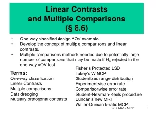
Linear Contrasts and Multiple Comparisons(Chapter 9) • One-way classified design AOV example. • Develop the concept of multiple comparisons and linear contrasts. • Multiple comparisons methods needed due to potentially large number of comparisons that may be made if Ho rejected in the one-way AOV test. Terms: Linear Contrasts Multiple comparisons Data dredging Mutually orthogonal contrasts Experimentwise error rate Comparisonwise error rate MCPs: Fisher’s Protected LSD Tukey’s W (HSD) Studentized range distribution Student-Newman-Keuls procedure Scheffe’s Method Dunnett’s procedure STA 6166 - MCP
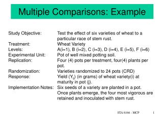
One-Way Layout Example A study was performed to examine the effect of a new sleep inducing drug on a population of insomniacs. Three (3) treatments were used: Standard Drug New Drug Placebo (as a control) What is the role of the placebo in this study? What is a control in an experimental study? 18 individuals were drawn (at random) from a list of known insomniacs maintained by local physicians. Each individual was randomly assigned to one of three groups. Each group was assigned a treatment. Neither the patient nor the physician knew, until the end of the study, which treatment they were on (double-blinded). Why double-blind? A proper experiment should be: randomized, controlled, and double-blinded. STA 6166 - MCP
Response: Average number of hours of sleep per night. Placebo: 5.6, 5.7, 5.1, 3.8, 4.6, 5.1 Standard Drug: 8.4, 8.2, 8.8, 7.1, 7.2, 8.0 New Drug: 10.6, 6.6, 8.0, 8.0, 6.8, 6.6 yij = response for the j-th individual on the i-th treatment. Hartley’s test for equal variances: Fmax = 4.77 < Fmax_critical = 10.8 STA 6166 - MCP
Excell Analysis Tool Output What do we conclude here? STA 6166 - MCP
Linear Contrasts and Multiple Comparisons If we reject H0 of no differences in treatment means in favor of HA, we conclude that at least one of the t population means differs from the other t-1. Which means differ from each other? Multiple comparison procedures have been developed to help determine which means are significantly different from each other. Many different approaches - not all produce the same result. Data dredging and data snooping - analyzing only those comparisons which look interesting after looking at the data – affects the error rate! Problems with the confidence assumed for the comparisons: 1-a for a particular pre-specified comparison? 1-a for all unplanned comparisons as a group? STA 6166 - MCP
Linear Comparisons Example: To compare m1 to m2 we use the equation: with coefficients Note constraint is met! Any linear comparison among t population means, m1, m2, ...., mt can be written as: Where the ai are constants satisfying the constraint: STA 6166 - MCP
Linear Contrast Variance of a linear contrast: Test of significance A linear comparison estimated by using group means is called a linear contrast. Ho: l = 0 vs. Ha: l 0 STA 6166 - MCP
Orthogonal Contrasts These two contrasts are said to be orthogonal if: in which case l1 conveys no information about l2 and vice-versa. A set of three or more contrasts are said to be mutually orthogonal if all pairs of linear contrasts are orthogonal. STA 6166 - MCP
Compare average of drugs (2,3) to placebo (1). Contrast drugs (2,3). Orthogonal Non-orthogonal Contrast Standard drug (2) to placebo (1). Contrast New drug (3) to placebo (1). STA 6166 - MCP
Drug Comparisons STA 6166 - MCP
Importance of Mutual Orthogonality Assume t treatment groups, each group having n individuals (units). • t-1 mutually orthogonal contrasts can be formed from the t means. (Remember t-1 degrees of freedom.) • Treatment sums of squares (SSB) can be computed as the sum of the sums of squares associated with the t-1 orthogonal contrasts. (i.e. the treatment sums of squares can be partitioned into t-1 parts associated with t-1 mutually orthogonal contrasts). t-1 independent pieces of information about the variability in the treatment means. STA 6166 - MCP
Example of Linear Contrasts Objective: Test the wear quality of a new paint. Treatments: Weather and wood combinations. Treatment Code Combination A m1 hardwood, dry climate B m2 hardwood, wet climate C m3 softwood, dry climate D m4 softwood, wet climate (Obvious) Questions: Q1: Is the average life on hardwood the same as average life on softwood? Q2: Is the average life in dry climate the same as average life in wet climate? Q3: Does the difference in paint life between wet and dry climates depend upon whether the wood is hard or soft? STA 6166 - MCP
MSE= 5 t= 4 n -t= 8 t Q1 Q1: Is the average life on hardwood the same as average life on softwood? Comparison: Estimated Contrast Test H0: l1 = 0 versus HA: l1 0 What is MSl1 ? Test Statistic: Rejection Region: Reject H0 if STA 6166 - MCP
Conclusion: Since F=29.4 > 5.32 we reject H0 and conclude that there is a significant difference in average life on hard versus soft woods. STA 6166 - MCP
MSE= 5 t= 4 n -t= 8 t Q2 Q2: Is the average life in dry climate the same as average life in wet climate? Comparison: Estimated Contrast Test H0: l2 = 0 versus HA: l2 0 Test Statistic: Rejection Region: Reject H0 if STA 6166 - MCP
Conclusion: Since F=0.6 < 5.32 we do not reject H0 and conclude that there is not a significant difference in average life in wet versus dry climates. STA 6166 - MCP
MSE= 5 t= 4 n -t= 8 t Q3 Q3: Does the difference in paint life between wet and dry climates depend upon whether the wood is hard or soft? Comparison: Estimated Contrast Test H0: l3 = 0 versus HA: l3 0 Test Statistic: Rejection Region: Reject H0 if STA 6166 - MCP
Conclusion: Since F=0 < 5.32 we do not reject H0 and conclude that the difference between average paint life between wet and dry climates does not depend on wood type. Likewise, the difference between average paint life for the wood types does not depend on climate type (i.e. there is no interaction). STA 6166 - MCP
The three are mutually orthogonal. SSl1 = MSl1 = 147 SSl2 = MSl2 = 3 SSl3 = MSl3 = 0 Treatment SS = 150 The three mutually orthogonal contrasts add up to the Treatment Sums of Squares. Total Error SS = dferror x MSE = 8 x 5 = 40 Mutual Orthogonality STA 6166 - MCP
(Type I) Error Rate STA 6166 - MCP
If Ho is true, and α=0.05, we can expect to make a Type I error 5% of the time… 1 out of every 20 will yield p-value<0.05, even though there is no effect! STA 6166 - MCP
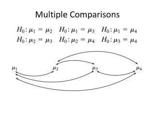
Types of Error Rates Compairsonwise Error Rate - the probability of making a Type I error in a single test that involves the comparison of two means. (Our usual definition of Type I error thus far…) Question: How should we define Type I error in an experiment (test) that involves doing several tests? What is the “overall” Type I error? The following definition seems sensible: Experimentwise Error Rate - the probability of observing an experiment in which one or more of the pairwise comparisons are incorrectly declared significantly different. This is the probability of making at least one Type I error. STA 6166 - MCP
Error Rates: Problems Suppose we make c mutually orthogonal (independent) comparisons, each with Type I comparisonwise error rate of a. The experimentwise error rate, e, is then: If the comparisons are not orthogonal, then the experimentwise error rate is smaller. Thus in most situations we actually have: STA 6166 - MCP
The Bonferroni Solution Solution: set e=0.05 and solve for : But there’s a problem… E.g. if c=8, we get =0.0064! Very conservative…, thus type II error is large. Bonferroni’s inequality provides an approximate solution to this that guarantees: We set: E.g. if c=8, we get =0.05/8=0.0063. Still conservative! STA 6166 - MCP
Multiple Comparison Procedures (MCPs): Overview • Terms: • If the MCP requires a significant overall F test, then the procedure is called a protected method. • Not all procedures produce the same results. (An optimal procedure could be devised if the degree of dependence, and other factors, among the comparisons were known…) • The major differences among all of the different MCPs is in the calculation of the yardstick used to determine if two means are significantly different. The yardstick can generically be referred to as the least significant difference. Any two means greater than this difference are declared significantly different. STA 6166 - MCP
Multiple Comparison Procedures: Overview • Yardsticks are composed of a standard error term and a critical value from some tabulated statistic. • Some procedures have “fixed” yardsticks, some have “variable” yardsticks. The variable yardsticks will depend on how far apart two observed means are in a rank ordered list of the mean values. • Some procedures control Comparisonwise Error, other Experimentwise Error, and some attempt to control both. Some are even more specialized, e.g. Dunnett’s applies only to comparisons of treatments to a control. STA 6166 - MCP
Fisher’s Least Significant Difference - Protected Mean of group i (mi) is significantly different from the mean of group j (mj) if if all groups have same size n. Type I (comparisonwise) error rate = a Controls Comparisonwise Error. Experimentwise error control comes from requiring a significant overall F test prior to performing any comparisons, and from applying the method only to pre-planned comparisons. STA 6166 - MCP
Tukey’s W (Honestly Significant Difference) Procedure Primarily suited for all pairwise comparisons among t means. Means are different if: {Table 10 - critical values of the studentized range.} Experimentwise error rate = a This MCP controls experimentwise error rate! Comparisonwise error rates is thus very low. STA 6166 - MCP
Student Newman Keul Procedure A modified Tukey’s MCP.Rank the t sample means from smallest to largest. For two means that are r “steps” apart in the ranked list, we declare the population means different if: {Table 10 - critical values of the studentized range. Depends on which mean pair is being considered!} varying yardstick r=6 r=5 r=2 r=3 r=4 STA 6166 - MCP
Duncan’s New Multiple Range Test (Passe) Number of steps Protection Level Probability of Apart, r (0.95)r-1 Falsely Rejecting H0 2 .950 .050 3 .903 .097 4 .857 .143 5 .815 .185 6 .774 .226 7 .735 .265 Neither an experimentwise or comparisonwise error rate control alone. Based on a ranking of the observed means. Introduces the concept of a “protection level” (1-a)r-1 {Table A -11 (later) in these notes} STA 6166 - MCP
Dunnett’s Procedure A MCP that is used for comparing treatments to a control. It aims to control the experimentwise error rate. Compares each treatment mean (i) to the mean for the control group (c). • dα(k,v) is obtained from Table A-11 (in the book) and is based on: • α = the desired experimentwise error rate • k = t-1, number of noncontrol treatments • v = error degrees of freedom. STA 6166 - MCP
Scheffé’s S Method For any linear contrast: Estimated by: With estimated variance: To test H0: l = 0 versus Ha: l ¹ 0 For a specified value of a, reject H0 if: where: STA 6166 - MCP
Adjustment for unequal sample sizes: The Harmonic Mean If the sample sizes are not equal in all t groups, the value of n in the equations for Tukey and SNK can be replaced with the harmonic mean of the sample sizes: E.g. Tukey’s W becomes: Or can also use Tukey-Cramer method: STA 6166 - MCP
MCP Confidence Intervals In some MCPs we can also form simultaneous confidence intervals (CI’s) for any pair of means, μi - μj. • Fisher’s LSD: • Tukey’s W: • Scheffe’s for a contrast I: STA 6166 - MCP
A Nonparametric MCP (§9.9) • The (parametric) MCPs just discussed all assume the data are random samples from normal distributions with equal variances. • In many situations this assumption is not plausible, e.g. incomes, proportions, survival times. • Let τi be the shift parameter (e.g. median) for population i, i=1,…,t. Want to determine if populations differ with respect to their shift parameters. • Combine all samples into one, rank obs from smallest to largest. Denote mean of ranks for group i by: STA 6166 - MCP
Nonparametric Kruskal-Wallis MCP This MCP controls experimentwise error rate. • Perform the Kruskall-Wallis test of equality of shift parameters (null hypothesis). • If this test yields an insignificant p-value, declare no differences in the shift parameters and stop. • If not, declare populations i and j to be different if STA 6166 - MCP
Comparisonwise error rates for different MCP STA 6166 - MCP
Experimentwise error rates for different MCP STA 6166 - MCP