Multiple Linear Regression and Correlation Analysis

1. Multiple Linear Regression and Correlation Analysis Chapter 14

2. GOALS • Describe the relationship between several independent variables and a dependent variable using multiple regression analysis. • Compute and interpret the multiple standard error of estimate, the coefficient of multiple determination, and the adjusted coefficient of multiple determination. • Conduct a test of hypothesis on each of the regression coefficients. • Use and understand qualitative independent variables.

3. Multiple Regression Analysis The general multiple regression with k independent variables is given by: The least squares criterion is used to develop this equation. Because determining b1, b2, etc. is very tedious, a software package such as Excel or MINITAB is recommended.

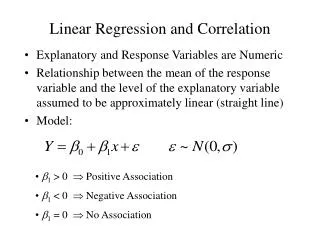
4. Multiple Regression Analysis For two independent variables, the general form of the multiple regression equation is: • X1 and X2 are the independent variables. • a is the Y-intercept • b1 is the net change in Y for each unit change in X1 holding X2 constant. It is called a partial regression coefficient, a net regression coefficient, or just a regression coefficient.

5. Regression Plane for a 2-Independent Variable Linear Regression Equation

6. Multiple Linear Regression - Example Salsberry Realty sells homes along the east coast of the United States. One of the questions most frequently asked by prospective buyers is: If we purchase this home, how much can we expect to pay to heat it during the winter? The research department at Salsberry has been asked to develop some guidelines regarding heating costs for single-family homes. Three variables are thought to relate to the heating costs: (1) the mean daily outside temperature, (2) the number of inches of insulation in the attic, and (3) the age in years of the furnace. To investigate, Salsberry’s research department selected a random sample of 20 recently sold homes. It determined the cost to heat each home last January, as well (data in next slide)

7. Multiple Linear Regression - Example

8. The Multiple Regression Equation – Interpreting the Regression Coefficients The regression coefficient for mean outside temperature (X1) is 4.583. The coefficient is negative and shows an inverse relationship between heating cost and temperature. As the outside temperature increases, the cost to heat the home decreases. The numeric value of the regression coefficient provides more information. If we increase temperature by 1 degree and hold the other two independent variables constant, we can estimate a decrease of $4.583 in monthly heating cost.

9. The Multiple Regression Equation – Interpreting the Regression Coefficients The attic insulation variable (X2) also shows an inverse relationship: the more insulation in the attic, the less the cost to heat the home. So the negative sign for this coefficient is logical. For each additional inch of insulation, we expect the cost to heat the home to decline $14.83 per month, regardless of the outside temperature or the age of the furnace.

10. The Multiple Regression Equation – Interpreting the Regression Coefficients The age of the furnace variable (X3) shows a direct relationship. With an older furnace, the cost to heat the home increases. Specifically, for each additional year older the furnace is, we expect the cost to increase $6.10 per month.

11. Applying the Model for Estimation What is the estimated heating cost for a home if the mean outside temperature is 30 degrees, there are 5 inches of insulation in the attic, and the furnace is 10 years old?

12. Multiple Standard Error of Estimate The multiple standard error of estimate is a measure of the effectiveness of the regression equation. • It is measured in the same units as the dependent variable. • It is difficult to determine what is a large value and what is a small value of the standard error. • The formula is:

14. Multiple Regression and Correlation Assumptions • The independent variables and the dependent variable have a linear relationship. The dependent variable must be continuous and at least interval-scale. • The residual must be the same for all values of Y. When this is the case, we say the difference exhibits homoscedasticity. • The residuals should follow the normal distribution with mean 0. • Successive values of the dependent variable must be uncorrelated.

15. The ANOVA Table The ANOVA table reports the variation in the dependent variable. The variation is divided into two components. • The Explained Variation is that accounted for by the set of independent variable. • The Unexplained or Random Variation is not accounted for by the independent variables.

16. Minitab – the ANOVA Table

17. Coefficient of Multiple Determination (r2) Characteristics of the coefficient of multiple determination: 1. It is symbolized by a capital R squared. In other words, it is written as because it behaves like the square of a correlation coefficient. 2. It can range from 0 to 1. A value near 0 indicates little association between the set of independent variables and the dependent variable. A value near 1 means a strong association. 3. It cannot assume negative values. Any number that is squared or raised to the second power cannot be negative. 4. It is easy to interpret. Because R2 is a value between 0 and 1 it is easy to interpret, compare, and understand.

18. Coefficient of Multiple Determination (r2)- Formula

19. Minitab – the ANOVA Table

20. Adjusted Coefficient of Determination • The number of independent variables in a multiple regression equation makes the coefficient of determination larger. • If the number of variables, k, and the sample size, n, are equal, the coefficient of determination is 1.0. • To balance the effect that the number of independent variables has on the coefficient of multiple determination, statistical software packages use an adjusted coefficient of multiple determination.

21. Adjusted Coefficient of Determination - Example

22. Correlation Matrix A correlation matrix is used to show all possible simple correlation coefficients among the variables. • The matrix is useful for locating correlated independent variables. • It shows how strongly each independent variable is correlated with the dependent variable.

23. Global Test: Testing the Multiple Regression Model The global test is used to investigate whether any of the independent variables have significant coefficients. The hypotheses are:

24. Global Test continued • The test statistic is the F distribution with k (number of independent variables) and n-(k+1) degrees of freedom, where n is the sample size. • Decision Rule: Reject H0 if F > F,k,n-k-1 Or in SPSS when in ANOVA table; p-value<.05

25. Interpretation • The computed F is 21.90, or When p-value<.05, so we can reject H0 • The null hypothesis that all the multiple regression coefficients are zero is therefore rejected. • Interpretation: some of the independent variables (amount of insulation, etc.) do have the ability to explain the variation in the dependent variable (heating cost).

26. Evaluating Individual Regression Coefficients (βi = 0) • Test is used to determine which independent variables have nonzero regression coefficients. • The variables that have zero regression coefficients are usually dropped from the analysis. • The test statistic is the t distribution with n-(k+1) degrees of freedom. • The hypothesis test is as follows: H0: βi = 0 H1: βi ≠ 0 Reject H0 if p-value<.05 or T-value (approximately greater than 2.0)

27. Critical t-stat for the Slopes

28. Computed t-stat for the Slopes

29. New Regression Model without Variable “Age” – Minitab P-value<.05

30. New Regression Model without Variable “Age” – Minitab

31. Testing the New Model for Significance

32. Critical t-stat for the New Slopes

33. Evaluating theAssumptions of Multiple Regression 1. There is a linear relationship. That is, there is a straight-line relationship between the dependent variable and the set of independent variables. 2. The variation in the residuals is the same for both large and small values of the estimated YTo put it another way, the residual is unrelated whether the estimated Y is large or small. 3. The residuals follow the normal probability distribution. 4. The independent variables should not be correlated. That is, we would like to select a set of independent variables that are not themselves correlated. 5. The residuals are independent. This means that successive observations of the dependent variable are not correlated. This assumption is often violated when time is involved with the sampled observations.

34. Analysis of Residuals A residual is the difference between the actual value of Y and the predicted value of Y. Residuals should be approximately normally distributed. Histograms and stem-and-leaf charts are useful in checking this requirement. • A plot of the residuals and their corresponding Y’ values is used for showing that there are no trends or patterns in the residuals.

35. Scatter Diagram

36. Residual Plot

37. Distribution of Residuals Both MINITAB and Excel offer another graph that helps to evaluate the assumption of normally distributed residuals. It is a called a normal probability plot and is shown to the right of the histogram.

38. Multicollinearity • Multicollinearity exists when independent variables (X’s) are correlated. • Correlated independent variables make it difficult to make inferences about the individual regression coefficients (slopes) and their individual effects on the dependent variable (Y). • However, correlated independent variables do not affect a multiple regression equation’s ability to predict the dependent variable (Y).

39. Effect of Multicollinearity in • Not a Problem: Multicollinearity does not affect a multiple regression equation’s ability to predict the dependent variable • A Problem: Multicollinearity may show unexpected results in evaluating the relationship between each independent variable and the dependent variable (a.k.a. partial correlation analysis),

40. Clues Indicating Problems with Multicollinearity • An independent variable known to be an important predictor ends up having a regression coefficient that is not significant. • A regression coefficient that should have a positive sign turns out to be negative, or vice versa. • When an independent variable is added or removed, there is a drastic change in the values of the remaining regression coefficients.

41. Variance Inflation Factor • A general rule is if the correlation between two independent variables is between -0.70 and 0.70 there likely is not a problem using both of the independent variables. • A more precise test is to use the variance inflation factor (VIF). • The value of VIF is found as follows: • The term R2j refers to the coefficient of determination, where the selected independent variable is used as a dependent variable and the remaining independent variables are used as independent variables. • A VIF greater than 10 is considered unsatisfactory, indicating that independent variable should be removed from the analysis.

42. Multicollinearity – Example Refer to the data in the table, which relates the heating cost to the independent variables outside temperature, amount of insulation, and age of furnace. Develop a correlation matrix for all the independent variables. Does it appear there is a problem with multicollinearity? Find and interpret the variance inflation factor for each of the independent variables.

43. Correlation Matrix - Minitab

44. Coefficient of Determination VIF – Minitab Example The VIF value of 1.32 is less than the upper limit of 10. This indicates that the independent variable temperature is not strongly correlated with the other independent variables.

45. Independence Assumption • The fifth assumption about regression and correlation analysis is that successive residuals should be independent. • When successive residuals are correlated we refer to this condition as autocorrelation. Autocorrelation frequently occurs when the data are collected over a period of time.

46. Residual Plot versus Fitted Values • The graph shows the residuals plotted on the vertical axis and the fitted values on the horizontal axis. • Note the run of residuals above the mean of the residuals, followed by a run below the mean. A scatter plot such as this would indicate possible autocorrelation.

47. Durbin–Watson statistic • The Durbin–Watson statistic is a test statistic used to detect the presence of autocorrelation in the residuals from a regression analysis. It is named after James Durbin and Geoffrey Watson. • If et is the residual associated with the observation at time t, then the test statistic is

48. Durbin–Watson statistic • Since d is approximately equal to 2(1-r), where r is the sample autocorrelation of the residuals, d = 2 indicates that appears to be no autocorrelation, its value always lies between 0 and 4. • If the Durbin–Watson statistic is substantially less than 2, there is evidence of positive serial correlation. As a rough rule of thumb, if Durbin–Watson is less than 1.0, there may be cause for alarm. • Small values of d indicate successive error terms are, on average, close in value to one another, or positively correlated. If d > 2successive error terms are, on average, much different in value to one another, i.e., negatively correlated. In regressions, this can imply an underestimation of the level of statistical significance.

49. Qualitative Independent Variables • Frequently we wish to use nominal-scale variables—such as gender, whether the home has a swimming pool, or whether the sports team was the home or the visiting team—in our analysis. These are called qualitative variables. • To use a qualitative variable in regression analysis, we use a scheme of dummy variablesin which one of the two possible conditions is coded 0 and the other 1.

50. Qualitative Variable - Example Suppose in the Salsberry Realty example that the independent variable “garage” is added. For those homes without an attached garage, 0 is used; for homes with an attached garage, a 1 is used. We will refer to the “garage” variable as X4.The data shown on the table are entered into the MINITAB system.