Data Analysis
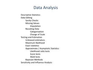
Data Analysis. Descriptive Statistics Data Editing Sanity Checks Missing Values Imputation Recoding Data Categorization Change of Scale Testing and Estimation Unbiased estimators Maximum likelihood Exact statistics Approximate / Asymptotic Statistics

Data Analysis
E N D
Presentation Transcript
Data Analysis Descriptive Statistics Data Editing Sanity Checks Missing Values Imputation Recoding Data Categorization Change of Scale Testing and Estimation Unbiased estimators Maximum likelihood Exact statistics Approximate / Asymptotic Statistics Likelihood ratio tests Score tests Wald tests Bayesian Methods Sensitivity and Influence Analysis
Descriptive Statistics and Data Editing Sanity Checks Check for impossible values Histograms and scatter plots are trends sensible are there outliers Missing Values Imputation Recoding Data Categorization Change of Scale
Descriptive Statistics and Data Editing Recoding Data Categorization Change of Scale Intercepts
Descriptive Statistics and Data Editing Missing Values Throw out records with missing values Imputation nearest neighbors model for missing value given available data
Testing and Estimation Testing and Estimation Maximum likelihood Exact statistics Approximate / Asymptotic Statistics Likelihood ratio tests Score tests Wald tests Bayesian Methods
Testing and Estimation Exact statistics not “exactly what you want” assumptions are made that allow calculation of effect sizes or p-values without using approximations like an assumption of normally distributed quantities. Assume observations come from a process that is simple enough to describe exactly with a tractable probability model -- Fisher’s Exact Test Permutation methods -- under the null hypothesis, there is no association between the exposure and outcome -- calculate the effect size somehow -- repeat many times * shuffle the values of the outcome variable * recalculate the effect size on permuted data * store the effect -- check how the actual effect size compares to the distribution of permuted effect estimates
Testing and Estimation Maximum likelihood
Testing and Estimation Approximate / Asymptotic Statistics Likelihood ratio tests Score tests Wald tests
Testing and Estimation Bayesian Methods probability as degree of knowledge Pr(A,B) = Pr(A|B)Pr(B) = Pr(B|A)Pr(A) Pr(B|A) = Pr(A|B)Pr(B) / Pr(A) Pr(model|data) = Pr(data|model) Pr(model) / Pr(data) posterior = likelihood * prior / normalization constant Use of prior: Some cases, similar to adding ½ count to each cell of a contingincy Table Push estimates toward “sensible values”
Testing and Estimation Testing and Estimation Unbiased estimators Maximum likelihood Exact statistics Approximate / Asymptotic Statistics Likelihood ratio tests Score tests Wald tests Bayesian Methods
Sensitivity and Influence Analysis Sensitivity Analysis All statistical techniques start with assumptions that cannot be confirmed with existing data One could run several analyses using different assumptions If the conclusions from a set of analyses are largely in agreement, then the conclusions are not SENSITIVE to the assumptions of the analyses If the results of the analyses are different, use results cautiously because they are based on unconfirmed assumptions Examples: Different statistical models Different estimation techniques Different corrections for selection bias Different corrections for misclassification
Sensitivity and Influence Analysis Influence Analysis Are a small number of observations determining the conclusions of a data analysis outliers
Bias Analysis Analysis of Unmeasured Confounders Selection Bias Analysis of Misclassification
Classification: Two levels Sensitivity = Pr(report exposure | true exposure ) = Pr(e=1 | E=1) Specificity = Pr(report not exposed | truly not exposed) = Pr(e=0 | E=0)
Classification or Prediction Sensitivity = Pr( report disease | true disease) Sensitivity = Pr( report exposure | true exposure) Sensitivity = Pr(event happens | predict that event will happen) Specificity = Pr(report no disease | truly no disease) Specificity = Pr(report no exposure | truly no exposure) Specificity = Pr(no event happens | predict that no event will happen)
Logistic Regression as Classifier After fitting a logistic regression model: For each individual used to fit the model, you can calculate a probability of having the outcome variable = 1 (radiation therapy instead of prostatectomy) You could use Pr(outcome = 1 ) = 0.5 as a cutoff: individuals with probabilities greater than the cutoff are assigned or predicted to be in the outcome=1 category; otherwise they are assigned or precicted to be in the outcome=0 category. By comparing these predictions to the actual outcomes, you can calculate sensitivities and specificities
Classification . logistic treat2 age race inst i.gleasoncat Logistic regression Number of obs = 330 LR chi2(5) = 93.73 Prob > chi2 = 0.0000 Log likelihood = -181.84698 Pseudo R2 = 0.2049 ------------------------------------------------------------------------------ treat2 | Odds Ratio Std. Err. z P>|z| [95% Conf. Interval] -------------+---------------------------------------------------------------- age | 1.14762 .0219378 7.20 0.000 1.105418 1.191433 race | 5.464351 2.101918 4.41 0.000 2.571078 11.61347 inst | .845149 .2970819 -0.48 0.632 .4243497 1.683227 | gleasoncat | 2 | .5591875 .2315788 -1.40 0.160 .2483394 1.259126 3 | .4410856 .1823707 -1.98 0.048 .196149 .9918811 ------------------------------------------------------------------------------
Errors in Measurements and Misclassification . estat classification Logistic model for treat2 -------- True -------- Classified | D ~D | Total -----------+--------------------------+----------- + | 113 44 | 157 - | 50 123 | 173 -----------+--------------------------+----------- Total | 163 167 | 330 Classified + if predicted Pr(D) >= .5 True D defined as treat2 != 0 -------------------------------------------------- Sensitivity Pr( +| D) 69.33% Specificity Pr( -|~D) 73.65% Positive predictive value Pr( D| +) 71.97% Negative predictive value Pr(~D| -) 71.10% -------------------------------------------------- False + rate for true ~D Pr( +|~D) 26.35% False - rate for true D Pr( -| D) 30.67% False + rate for classified + Pr(~D| +) 28.03% False - rate for classified - Pr( D| -) 28.90% -------------------------------------------------- Correctly classified 71.52% --------------------------------------------------
Classification You could try probability cutoffs other than 0.5. ROC curves: Try many cutoffs between Pr(outcome=1)=0 and Pr(outcome=1)=1 Calculate the sensitivity and specificity for each cutoff Plot Sensitivity vs 1-Specificity
Classification You could try probability cutoffs other than 0.5. ROC curves: Try many cutoffs between Pr(outcome=1)=0 and Pr(outcome=1)=1 Calculate the sensitivity and specificity for each cutoff Plot Sensitivity vs. 1-Specificity .lsens : plot sensitivity and specificity vs. cutoff .lroc : plot ROC curve Sensitivity and Specificity are inversely related The area under the curve (AUC) or the 2 times the area between the curve and the diagonal line (Gini coefficient) are used to assess the quality of the classifier/ prediction system Assess quality of classifier with data that was not used to generate/fit/train the classifier (cross validation)
Misclassification If you know the sensitivity and specificity for a classifier, you can work from their definitions to calculate the expected numbers of exposed and not exposed given the true numbers exposed and not exposed. Start by assuming a sensitivity (say 0.9) and specificity (say 0.95) and defining a vector of true counts v = [100, 100]:
Misclassification Then define a matrix as follows:
Misclassification Or based on the sensitivity and specificity given above: Call this matrix T. The expected counts of exposed and not exposed, based on the true counts of exposed and the transition matrix will be: verr = v * T
Misclassification Stata: . matrix v = [100,100] . matrix T = [.9, .1\.05,.95] . matrix list v v[1,2] c1 c2 r1 100 100 . matrix list T T[2,2] c1 c2 r1 .9 .1 r2 .05 .95
Misclassification Since the observed counts verr = v * T, we can recover the true counts v if we know or can assume T: 1: Use the matrix T to calculate its inverse Tinv 2: Multiply verr * Tinv = v * T * Tinv = v Stata: . matrix Tinv = inv(T) . matrix vadj = verr * Tinv . matrix list vadj vadj[1,2] r1 r2 r1 100 100
Misclassification Simulating or correcting misclassification of EITHER exposure or outcome is not hard. If both exposure and outcome can be misclassified, there is the additional issue of whether or not the two types of misclassification are independent Misclassification may depend on levels of other covariates as well
Misclassification “non-differential misclassification biases effect estimates towards the null”
Misclassification “non-differential misclassification biases effect estimates towards the null” -- for misclassification of variables with only TWO levels -- for independent observations -- with sufficiently low sensitivities and specificities, you can get stronger effect sizes … but in the opposite direction
Misclassification Misclassification is measurement error for categorical variables There can be and probably is measurement error in any continuous variables you may use -- measurement error in independent variables is usually ignored
Unmeasured Confounders and Selection Bias Unmeasured Confounders External Adjustment Selection Bias: Weight observations by 1/selection probability
Selection Bias Text

