Download
1 / 61
610 likes | 797 Views
Onto 3D. Coordinate systems 3-D homogeneous transformations Translation, scaling, rotation Changes of coordinates Rigid transformations. Vector Projection. The projection of vector a onto u is that component of a in the direction of u. Vector Cross Product.

E N D
Onto 3D • Coordinate systems • 3-D homogeneous transformations • Translation, scaling, rotation • Changes of coordinates • Rigid transformations Computer Vision : CISC4/689
Vector Projection • The projection of vector a onto u is that component of a in the direction of u Computer Vision : CISC4/689
Vector Cross Product • Definition: If a=(xa, ya, za)T and • b=(xb, yb, zb)T, then: c=aXb c is orthogonal to both aand b Computer Vision : CISC4/689 from Hill
Coordinate System: Definitions • Let x=(x, y, z)T be a point in 3-D space (R3). What do these values mean? • A coordinate system in Rn is defined by an origin o and n orthogonal basis vectors • In R3, positive direction of each axis X, Y, Z is indicated by unit vector i, j, k, respectively, where k=iXj(in a right-handed system) • Coordinate is length of projection of vector from origin to point onto axis basis vector—e.g., x= x ¢ i o x Computer Vision : CISC4/689
3-D Camera Coordinates • Right-handed system • From point of view of camera looking out into scene: • +X right, {X left • +Y down, {Y up • +Zin front of camera, {Z behind Computer Vision : CISC4/689
Going from 2-D to 3-D • Points: Add z coordinate • Transformations: Become 4 x 4 matrices with extra row/column for z component—e.g., translation: Computer Vision : CISC4/689
3-D Scaling Computer Vision : CISC4/689
3-D Rotations • In 2-D, we are always rotating in the plane of the image, but in 3-D the axis of rotation itself is a variable • Three canonical rotation axes are the coordinate axes X, Y, Z • These are sometimes referred to • in aviation terms: pitch, yaw or heading, and roll, respectively from Hill Pitch is the angle that its longitudinal axis (running from tail to nose and along n) makes with horizontal plane. Computer Vision : CISC4/689 from Hill
3-D Euler Rotation Matrices • Similar to 2-D rotation matrices, but with coordinate corresponding to rotation axis held constant • E.g., a rotation about the X axis of µ radians: Computer Vision : CISC4/689
3-D Rotation Matrices • General form is: • Properties • RT= R-1 • Preserves vector lengths, angles between vectors • Upper-left block R3£3 is orthogonal matrix • Rows form orthonormal basis (as do columns): Length = 1, mutually orthogonal • So R3£3x projects point x onto unit vectors represented by rows of R3£3 Computer Vision : CISC4/689
Coordinate System Conversion • Camera coordinates C: Origin at center of camera, Z axis pointed in viewing direction • World coordinates W: Arbitrary origin, axes • Way to specify camera location, orientation (aka pose) in same frame as scene objects (we like to move camera to world, so as to convert world coordinates into camera coordinates) • Cx,Wx,: Same point in different coordinates Computer Vision : CISC4/689
Coordinate System Conversion • Camera coordinates C: Origin at center of camera, Z axis pointed in viewing direction • World coordinates W: Arbitrary origin, axes • Way to specify camera location, orientation (aka pose) in same frame as scene objects • Cx,Wx,: Same point in different coordinates Computer Vision : CISC4/689
Coordinate System Conversion • Camera coordinates C: Origin at center of camera, Z axis pointed in viewing direction • World coordinates W: Arbitrary origin, axes • Way to specify camera location, orientation (aka pose) in same frame as scene objects • Cx,Wx,: Same point in different coordinates Computer Vision : CISC4/689
Change of Coordinates: Special Case of Same Axes • Distinct origins, parallel basis vectors: If B is world, Ax (camera) can be obtained by Bx (world) minus its CG. Computer Vision : CISC4/689
Change of Coordinates: Special Case of Same Origin • Just need to rotate basis vectors so that they are aligned • Rotation matrix is projection of basis vectors in new frame ia ib ja 0 ka 0 ia 0 ja jb ka 0 ia 0 ja 0 ka kb Check by multing (ib 0 0), etc. i.e, take A coordinate system As (1 0 0), (0 1 0), (0 0 1) Computer Vision : CISC4/689
3-D Rigid Transformations • Combination of rotation followed by translation without scaling • “Moves” an object from one 3-D position and orientation (pose) to another T R M Computer Vision : CISC4/689
3-D Transformations: Arbitrary Change of Coordinates • A rigid transformation can be used to represent a general change in the coordinate system that “expresses” a point’s location Computer Vision : CISC4/689
Rigid Transformations: Homogeneous Coordinates • Points in one coordinate system are transformed to the other as follows: • takes the camera to the world origin, transforming world coordinates to camera coordinates • If A is camera and B is world, inverse translation and inverse rotation Computer Vision : CISC4/689
Camera Projection Matrix • Using homogeneous coordinates, we can describe perspective projection as the result of multiplying by a 3 x 4 matrix P: (by the rule for converting between homo-geneous and regular coordinates—this is perspective division) Computer Vision : CISC4/689
Camera Projection Matrix: Image Offsets Center of CCD matrix usually does not coincide with the principal point C0. This adds u0 and v0 to define in pixel units of C0 in retinal coordinate system. Computer Vision : CISC4/689
Factoring the Camera Matrix • Another way to write it: P=K ( Id 0 ) Camera calibration matrix Identity form of rigid transformation (with 4th row dropped) Computer Vision : CISC4/689
Camera Calibration Matrix • More general matrix allows: • Image coordinates with an offset origin (e.g., convention of upper left corner) • Non-square pixels = Different effective horizontal vs. vertical focal length • These four variables are known as the camera’s intrinsic parameters fu=f*su fv=f*sv Computer Vision : CISC4/689
Dealing with World Coordinates • Thus far we have assumed that points are in camera coordinates • Recall the definition of the world-to-camera coordinate rigid transformation: • In simpler form: Computer Vision : CISC4/689
Combining Intrinsic & Extrinsic Parameters • The transformation performed by a pinhole camera on an arbitrary point in world coordinates can be written as: 3 x 4 projective camera matrix P has 10 degrees of freedom (DOF): 4 intrinsic, 3 rotation, 3 translation Computer Vision : CISC4/689
Skew ignored • The textbook has skew parameter included (pp. 29). • Since the camera coordinate system may also be skewed due to some manufacturing error, the angle between the two image axes is not equal (maybe close to 90 degrees). This adds up another unknown parameter • Easy to incorporate, just makes it 11 unknowns Computer Vision : CISC4/689
Applications • Estimates of the camera matrix parameters are critical in order to: • Know where the camera is and how it is moving • Deduce structural characteristics of the scene (i.e., 3-D information) • Place known objects (e.g., computer graphics) into a camera image correctly Computer Vision : CISC4/689
Camera Matrix • Linear systems of equations • Least-squares estimation • Application: Estimating the camera matrix Computer Vision : CISC4/689
Linear System • A general set of m simultaneous linear equations in n variables can be written as: Computer Vision : CISC4/689
Matrix Form of Linear System • This can be represented as a matrix-vector product: • Compactly, we write this as Ax = b Computer Vision : CISC4/689
Solving Linear Systems • If m=n (A is a square matrix), then we can obtain the solution by simple inversion: • If m>n, then the system is over-constrained and Ais not invertible • Use the pseudoinverse A+ =(ATA)-1AT to obtain least-squares solutionx= A+b (Ax=B, multiply both sides by A^t, etc.) Computer Vision : CISC4/689
Fitting Lines • A 2-D point x = (x, y) is on a line with slope m and intercept b if and only if y =mx + b • Equivalently, • So the line defined by two points x1, x2 is the solution to the following system of equations: Computer Vision : CISC4/689
Fitting Lines • With more than two points, there is no guarantee that they will all be on the same line • Least-squares solution obtained from pseudoinverse is line that is “closest” to all of the points Computer Vision : CISC4/689 courtesy of Vanderbilt U.
Example: Fitting a Line • Suppose we have points (2, 1), (5, 2), (7, 3), and (8, 3) • Then and x = A+b =(0.3571, 0.2857)T Computer Vision : CISC4/689
Example: Fitting a Line Computer Vision : CISC4/689
Homogeneous Systems of Equations • Suppose we want to solve Ax = 0 • There is a trivial solution x = 0, but we don’t want this. For what other values of x is Ax close to 0? • This is satisfied by computing the singular value decomposition (SVD) A = UDVT (a non-negative diagonal matrix between two orthogonal matrices) and taking x as the last column of V (unit singular vector corresponding to the least eigenvalue. • Note that Matlab returns [U, D, V] = svd(A) This is usually subject to constraints such as norm of x=1 Computer Vision : CISC4/689
Line-Fitting as a Homogeneous System • A 2-D homogeneous point x = (x, y, 1)T is on the line l = (a, b, c)T only when ax + by + c = 0 • We can write this equation with a dot product: x¢l = 0,and hence the following system is implied for multiple points x1, x2, ..., xn: Computer Vision : CISC4/689
Example: Homogeneous Line-Fitting • Again we have 4 points, but now in homogeneous form: (2, 1, 1), (5, 2, 1), (7, 3, 1), and (8, 3, 1) • Our system is: • Taking the SVD of A, we get: b=-1, a=.3571, c=0.2857..scaled differently C ompare tox =(0.3571, 0.2857)T Computer Vision : CISC4/689
Camera Calibration • Camera calibration is the name given to the process of discovering the projection matrix (and its decomposition into camera matrix and the position and orientation of the camera) from an image of a controlled scene. For ex., we might set up the camera to view a calibrated grid of some sort. Computer Vision : CISC4/689
A Vision Problem: Estimating P • Given a number of correspondences between 3-D points and their 2-D image projections Xi$ xi, we would like to determine the camera projection matrixP such that xi =PXifor all i Computer Vision : CISC4/689
Y xi Xi Z X A Calibration Target Computer Vision : CISC4/689 courtesy of B. Wilburn
Estimating P: The Direct Linear Transformation (DLT) Algorithm • xi =PXiis an equation involving homogeneous vectors (powers are equal), so PXi and xi need only be in the same direction, not strictly equal • We can specify “same directionality” by using a cross product formulation: Computer Vision : CISC4/689
DLT Camera Matrix Estimation: Preliminaries • Let the image point xi = (xi, yi, wi)T (remember that Xi has 4 elements) • Denoting the jth row of P by pjT (a 4-element row vector), we have: Computer Vision : CISC4/689
DLT Camera Matrix Estimation: Step 1 • Then by the definition of the cross product, xi £PXi is: Definition of cross product: U x V = uy vz – uz vy, uz vx – ux vz, ux vy – uy vx Computer Vision : CISC4/689
DLT Camera Matrix Estimation: Step 2 • The dot product commutes, so pjTXi=XTipj, and we can rewrite the preceding as: Computer Vision : CISC4/689
DLT Camera Matrix Estimation: Step 3 • Collecting terms, this can be rewritten as a matrix product: where 0T = (0, 0, 0, 0). This is a 3 x 12 matrix times a 12-element column vector p = (p1T, p2T, p3T)T Computer Vision : CISC4/689
What We Just Did Computer Vision : CISC4/689
DLT Camera Matrix Estimation: Step 4 • There are only two linearly independent rows here • The third row is obtained by adding xi times the first row to yi times the second and scaling the sum by -1/wi Computer Vision : CISC4/689
DLT Camera Matrix Estimation: Step 4 • So we can eliminate one row to obtain the following linear matrix equation for the ith pair of corresponding points: • Write this as Aip = 0 Computer Vision : CISC4/689
DLT Camera Matrix Estimation: Step 5 • Remember that there are 11 unknowns which generate the 3 x 4 homogeneous matrix P (represented in vector form by p) • Each point correspondence yields 2 equations (the two rows of Ai) • We need at least 5 ½ point correspondences to solve for p • Stack Ai to get homogeneous linear system Ap = 0 Computer Vision : CISC4/689
Direct Linear Transform (DLT) (summary) rank-2 matrix Computer Vision : CISC4/689