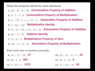
Download
1 / 12
120 likes | 205 Views
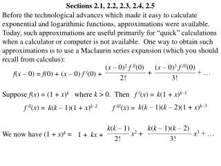
Sections 2.1, 2.2, 2.3, 2.4, 2.5.

E N D
Sections 2.1, 2.2, 2.3, 2.4, 2.5 Before the technological advances which made it easy to calculate exponential and logarithmic functions, approximations were available. Today, such approximations are useful primarily for “quick” calculations when a calculator or computer is not available. One way to obtain such approximations is to use a Maclaurin series expansion (which you should recall from calculus): (x– 0)2f(0) —————– + 2! (x– 0)3f(0) —————– + … 3! f(x– 0) = f(0) + (x– 0) f(0) + Suppose f(x) = (1 + x)k where k > 0. Then f(x) = f(x) = f(x) = We now have (1 + x)k = k(1 + x)k–1 k(k– 1)(k – 2)(1 + x)k–3 k(k– 1)(1 + x)k–2 k(k– 1) ——— x2 + 2! k(k– 1)(k– 2) —————— x3 + … 3! 1 + kx +
Suppose f(x) = ekx where k > 0. Then f(x) = f(x) = f(x) = We now have ekx = kekx k3ekx k2ekx k2 — x2 + 2! k3 — x3 + … 3! 1 + kx + From the previously derived expansions, we may write the following: k(k– 1) k(k– 1)(k– 2) (1 + i)k = 1 + ki + ——— i2 + —————— i3 + … 2! 3! (if k is a positive integer, this is a binomial expansion) (if k is not an integer, this is an infinite series expansion) (k)2 (k)3 ek = 1 + k + —— + —— + … 2! 3!
Using only the first two terms in one of these expansions (i.e., terms up to the first degree) would be considered a linear approximation; using only the first three terms in one of these expansions (i.e., terms up to the second degree) would be considered a quadratic approximation. Find the accumulated value of $4000 invested for three years at 7.4% convertible semiannually, by using (a) an exact calculation, (b) linear approximation, (c) quadratic approximation. 4000(1 + 0.037)6 = $4974.31 4000(1 + 0.037)6 4000(1 + 6(0.037)) = $4888.00 (Note that this is the same as using simple interest!) (3)(5) 4000(1 + 0.037)6 4000 1 + 6(0.037) + ———(0.037)2 = $4970.14 2
Find the accumulated value of $4000 invested for three years with a force of interest of 7.4%, by using (a) an exact calculation, (b) linear approximation, (c) quadratic approximation. 4000e(3)(0.074) = $4994.29 4000e(3)(0.074) = 4000e0.222 4000(1 + 0.222)) = $4888.00 (Note that this is like using simple interest with i = .) (0.222)2 4000e0.222 4000 1 + 0.222 + ——— = $4986.57 2
Suppose $4000 is invested at 7.4% per annum, and we would like the to find the value of the investment at 3.75 years. An exact answer could be found by obtaining 4000(1 + 0.074)3.75. An approximation could be obtained by using linear interpolation. In general, suppose k (0 < k < 1) represents the fraction of the period desired between periods n and n + 1. Linear interpolation yields the following approximation: (1 + i)n+k (1 –k)(1 + i)n + k(1 + i)n + 1 = (1 + i)n[(1 –k) + k(1 + i)] = (1 + i)n(1 + ki) This is the same as using simple interest over the final fractional period.
Find the accumulated value of $4000 invested for 3.75 years at 7.4% per annum, by using (a) an exact calculation, (b) linear interpolation. 4000(1 + 0.074)3.75 = $5227.89 4000(1 + 0.074)3(1 + (0.75)(0.74)) = $5230.35
Three commonly encountered (but not the only) methods for counting days in a period of investment: The “actual/actual” method is to use the exact number of days for the period of investment and to use 365 days in a year. (The table in Appendix II (page 393) is useful with this method.) Simple interest computed with this method is called exact simple interest. The “30/360” method is to assume that each calendar month has 30 days and that the calendar year has 360 days. Simple interest computed with this method is called ordinary simple interest. The number of days between two given dates can be found by using 360(Y2–Y1) + 30(M2–M1) + (D2–D1) where Y1 = year of first date Y2 = year of second date, M1 = month of first date M2 = month of second date D1 = day of first date D2 = day of second date The “actual/360” method is to use the exact number of days for the period of investment but to use only 360 days in a year. Simple interest computed with this method is called the Banker’s Rule.
(A “30/actual” method or a “30/365” method could be defined, but rarely is either one of these used in practice.) • Suppose that $2500 is deposited on March 8 and withdrawn on October 3 of the same year, and that the interest rate is 5%. Find the amount of interest earned, if it is computed using • exact simple interest, • (b) ordinary simple interest, • (c) the Banker’s Rule. With the help of Appendix II, 209 we obtain 2500 (0.05) —— = $71.58 . 365 First we obtain the number of days from 30(10–3) + (3–8) = 205. 205 Then, we obtain 2500 (0.05) —— = $71.18 . 360 With the counting done in part (a), 209 we obtain 2500 (0.05) —— = $72.60 . 360
Interest problems generally involve four quantities: principal(s), investment period length(s), interest rate(s), accumulates value(s). Two or more amounts of money payable at different points in time cannot be compared until a common date, called the comparison date, is established. An equation of value accumulates or discounts each payment to the comparison date. (A time diagram can be helpful in setting up an equation of value.) With compound interest, an equation of value will produce the same answer for an unknown value regardless of what comparison date is selected; however, this is not necessarily true for other patterns of interest.
In return for a payment of $1200 at the end of 10 years, a lender agrees to pay $200 immediately, $400 at the end of 6 years, and a final amount at the end of 15 years. Find the amount of the final payment at the end of 15 years if the nominal rate of interest is 9% converted semiannually. Time Diagram: $200 $400 $X Lender Borrower 0 1 2 3 4 5 6 7 8 9 10 11 12 13 14 15 $1200 (Time periods are counted in half-years, since interest is converted semiannually.) Equation of Value: v = 1 / (1 + 0.045) 200 + 400v12 + Xv30 = 1200v20
1200v20– 200 – 400v12 X = ————————— = v30 $231.11
In return for a payments of $5000 at the end of 3 years and $4000 at the end of 9 years, an investor agrees to pay $1500 immediately and to make an additional payment at the end of 2 years. Find the amount of the additional payment if i(4) = 0.08. $1500 $X Time Diagram: Investor Borrower 0 1 2 3 4 5 6 7 8 9 10 $5000 $4000 Equation of Value: (Time periods are counted in quarter-years, since interest is converted quarterly.) v = 1 / (1 + 0.02) 1500 + Xv8 = 5000v12 + 4000v36 X = $5159.24