Download
1 / 49
490 likes | 679 Views
GMI assessments of Aerosol–Cloud-Climate Interactions. 1 Donifan Barahona, 2 Rafaella Sotiropolou, and 1,2 Athanasios Nenes 1 Earth & Atmospheric Sciences, 2 Chemical & Biomolecular Engineering Georgia Institute of Technology.

E N D
GMI assessments of Aerosol–Cloud-Climate Interactions 1Donifan Barahona, 2Rafaella Sotiropolou, and 1,2Athanasios Nenes 1Earth & Atmospheric Sciences, 2Chemical & Biomolecular Engineering Georgia Institute of Technology
GMI assessments of Aerosol–Cloud-Climate Interactions:Current Work(Rafaella Sotiropoulou) Acknowledgements: NASA NIP, NASA IDS
GMI: Aerosol-Cloud-Climate Interactions Implementation of aerosol-cloud interaction modules: Cloud-relevant parameters change with meteo-fields used. Meteo-fields currently used: DAO, GISS, GEOS-4. Cloud properties are calculated from parameterizations. Implemented droplet formation parameterizations: Boucher and Lohmann, 1995 (BL) – empirical Abdul-Razzak & Ghan, 2000 (AG) - mechanistic Nenes & Seinfeld,2003; Fountoukis & Nenes,2005 (FN) – mechanistic Segal & Khain, 2006 (SK) - empirical Assessments of indirect effect and autoconversion rate using various droplet formation parameterization and meteorology. U of Michigan, AEROCOM aerosol emission scenarios. Currently Accomplished:
New GMI Improvements (since last meeting): Implementation of the CLIRAD-SW solar radiative transfer model (Chou et al., 1998; Chou and Suarez, 1999) online to calculate the cloud optical depth (COD) and shortwave (SW) cloud forcing from the surface layer to the top of the atmosphere (TOA). Aerosol indirect forcing (IF) is computed offline as the difference in the TOA net whole-sky shortwave flux (downwelling minus upwelling) between simulations that use present-day (PD; natural plus anthropogenic) and pre-industrial (PI; natural only) emissions. Repetition of all simulations
Simulations completed (since last mtg.) Emission Scenarios University of Michigan (Present day, Preindustrial) AEROCOM (Present day, Preindustrial) Base Case Simulations Liquid Cloud Temperatures: 273 K and above Cloud droplet formation schemes: BL and FN Sensitivity examined Cloud temperatures: 263 K over land, 269 K over ocean (GISS GCM scheme) Cloud droplet formation schemes: BL, SK, AG, FN Total Number of Simulations (for now): 4 3 2 2 + 4 3 2 = 72 AEROCOM U of Michigan Nd scheme Nd scheme Met field Threshold T Emission Case Met field Emission Case Results are presented for some of the sensitivity simulations
Annual Mean First IndirectForcing (W m-2) The spatial patterns of indirect forcing follow that of CDNC Spatially, there are strong horizontal inhomogeneities with the largest values of IF predicted over SE Asia, Western Europe and Eastern US (i.e., areas with highest amount of anthropogenic sulfur emissions) Range: -0.59 to -1.69 Wm-2 Sotiropoulou et al., ACPD Sotiropoulou et al, in prep
Annual Mean Autoconversion Forcing (%) Presindustrial Autoconversion Present day Autoconversion Autoconversion Forcing Large forcing over the continents and the ocean of the NH coinciding spatially with regions affected by pollution plumes or long range transport of pollution plumes. Autoconversion with Khairoutdinov and Kogan, 2000 Sotiropoulou et al, in prep
Implications and Conclusions GMI is able to correctly capture the land-ocean contrast in COD and reff and the spatial variations in cloud properties between the SH and the NH regions observed in remotely sensed data. Depending on the droplet activation parameterization and the metfield used, global annual indirect forcing ranges from -0.59 to -1.69 W m-2 for all runs considered to date Different metfields lead up to 40% (Global average) variability in indirect forcing calculations. Diagnostic and empirical parameterizations contribute up to 60% (Global average) variability in indirect forcing. Although important it is a low estimate (it becomes larger if you use interactive microphysics - our experience with CACTUS and CACTUS/TOMAS support this).
For all droplet activation parameterizations and the metfields used the global annual autoconversion rate ranges from 1.1010-11 to 10.3810-11 s-1 .The metfields contribute 70% variability and 30% is from the activation parameterization. The spatial patterns of autoconversion rate are similar for all metfields. Large differences in autoconversion rates over the oceans; this is one of the most important source of uncertainty from the droplet schemes. Larger autoconversion forcing (60-100%) is predicted over the anthropogenically perturbed regions of the globe Implications and Conclusions
GMI assessments of Aerosol–Cloud-Climate Interactions:Current WorkDonifan Barahona Acknowledgements: NASA NIP, NASA IDS
Cloud Droplet Formation in GCMs Current State-of-the-Art Cloud droplets • State-of-the-art: Physically-based prognostic representations of the activation physics. • Cloud droplet formation is parameterized by applying conservation principles in an ascending adiabatic air parcel. • All parameterizations developed to date rely on the assumption that the droplet formation is an adiabatic process. CCN Activation Height Aerosol particles in an closed adiabatic parcel Parcel Supersaturation
Peng, Y. et al. (2005). JGR In-situ data for marine clouds in N.Atlantic Adiabatic region Entraining region But…Real Clouds are NOT Adiabatic • Entrainment of air into cloudy parcels decreases droplet number relative to adiabatic conditions • In-situ observations often show that the liquid water content measured is lower than expected by adiabaticity. Neglecting entrainment may lead to an overestimation of in-cloud droplet number biasing indirect effect assessments
Barahona and Nenes (JGR, 2007)Entraining Cloud Droplet Parameterization Cloud droplets CCN Activation RH, T’ • Analytical formulation based on entraining air parcel framework: mixing of outside air is allowed • “Outside” air with (RH, T’) is assumed to entrain at a rate of e (kg air)(kg parcel)-1(m ascent)-1 • Can treat all the chemical complexities of organics, for either lognormal, sectional aerosol. Equally fast as adiabatic formulation. • Evaluated against detailed a numerical parcel model with average error below 3 ± 25 % • Will be evaluated with in-situ data (CIRPAS TO datasets) soon
V=5.0ms-1 Answer: around here (Controls droplet number) V=1.0ms-1 V=0.1ms-1 Entrainment Rate Critical (cloud completely evaporates) ~ Adiabatic When is Entrainment Important for Droplet Formation? • A “critical entrainment rate”, ec , exists for which mixing of outside air completely evaporates the cloud. • Entrainment becomes important if it is > 0.1 ec • Observation show that e varies from 0.0 to 0.6ec • Average for marine stratocumulus during MASE is 0.4ec (Wang et al. in review) Barahona and Nenes, 2007, JGR
GMI Implementation: Global distributions of Critical Entrainment Average ec is close but larger than reported values for e (~1-2 km-1) (i.e., Raga, et. al.; 1990) ec is higher in regions of high relative humidity, i.e., effect of entrainment is more important in dry (climatically sensitive) areas. Mean ec ~ 2.7 km-1 RH Present day simulations, GISS meteorology, annual averages
Entrainment Effects on Cloud Droplet Number e=0.4ec – Adiab. ~ -8% Adiabatic ~ 97 cm-3 e=0.6ec – Adiab. ~ -14% Up to 40% CDNC reduction in the tropics (larger effect on clean environments) Linking e to TKE may produce even more variability in CDNC. Present day, GISS meteorology, annual averages
Entrainment Impacts on Effective Radius e=0.4ec - Adiabatic = 0.16 μm Adiabatic ~ 7.78 μm e=0.6ec - Adiabatic = 0.32 μm Larger differences in the tropics (high LWC and Smax) ~ 1mm changes in large areas of the globe – important for IE Impacts on autoconversion rate are also important Present day, GISS meteorology, annual averages
Implications for Indirect Forcing e=0.4ec - Adiabatic = 0.11 Wm-2 Adiabatic = -1.28 Wm-2 e=0.6ec - Adiabatic = 0.22 Wm-2 Pattern follows Reff and LWC rather than droplet number Decreases indirect forcing by up to 20% Regional effects may be much larger (locally, up to 50%) Present day, GISS meteorology, annual averages
Ongoing Work • Obtaining entrainment rate from LWC and TKE fields either from GMI fields – when available – or from GISS runs using the model in our group (find a “global” e/ec). • Entrainment effects on autoconversion and accretion (and the list goes on…) • Sensitivity to all of the above with respect to GMI meteorological fields, aerosol microphysics, emission scenarios, etc. • Once the entrainment work is “finalized”, we will work with Jules to incorporate it in the “core” code at Goddard. Sorry Jules… (Thanos)
GMI assessments of Aerosol–Cloud-Climate Interactions:Future WorkIncluding Ice Microphysics Acknowledgements: NASA NIP, NASA IDS
http://www.alanbauer.com The importance of Cirrus Clouds • Cirrus are important for: • Radiative transfer: they tend to warm • Affecting stratospheric moisture • Regulation of the ocean temperature • Stratospheric circulation • Heterogeneous chemistry Cirrus may be affected by aircraft emissions, transport of dust and pollution. One of the initial motivations for GMI Aerosol effects on cirrus (and climate) are highly unknown!!
+ Ice Crystals RH, T, V Ice Germ Homogeneous Heterogeneous Liquid droplets + Insoluble material Modeling Cirrus Formation • Need to describe: • Onset of freezing • Ice crystal and droplet growth • Evolution of size distributions, RH and T • Challenges: • Size and composition effects, • role of dynamic variability, • heterogeneous nucleation, • deposition coefficient
Barahona and Nenes Ice Parameterization (JGR, in press) Parcel Saturation • The probability of freezing changes with time (unlike with liquid cloud droplet formation!) • Because of this, we need to trace back in time the growth of each ice crystal to find the conditionsat which freezing occurred. Ice Crystal So’ Instant of freezing time
Analytical Development of the Parameterization Find a Solution of:
Analytical Development of the Parameterization Find a Solution of:
Analytical Development of the Parameterization Find a Solution of: Calculate freezing probability:
Analytical Development of the Parameterization Find a Solution of: Calculate freezing probability: Calculate size distribution:
Analytical Development of the Parameterization Find a Solution of: Calculate freezing probability: Calculate size distribution: Integrate size distribution !
Analytical Development of the Parameterization Find a Solution of: LOTS AND LOTS OF MATH….. Calculate freezing probability: Calculate size distribution: Integrate size distribution !
Analytical Development of the Parameterization After all this effort … the parameterization reduces to: Ice Crystal Number Concentration 1-2 lines of FORTRAN code … but it is completely theoretical (i.e. rigorous and robust) and captures the (complex) physics of ice nucleation. We can also calculate the size distribution… (not shown)
Parameterization vs. Parcel Model Deposition coefficient 1200 runs. T= 200-235 K, V=0.02-5 ms-1. • Explicity considers effect of aerosol size and number, deposition coefficient, T, P, and updraft velocity. • Very robust: average error ~ 3 ± 28% • MANY orders of mangitude faster than parcel model Barahona and Nenes, JGR, in press
Barahona SB2000 KL2002 Parcel Model LP2005 (only for a=1) Comparison with other parameterizations Deposition Coefficient: Blue: 1.0 Black: 0.1 T=213K, No=200 cm-3 Ddry=40 nm Barahona and Nenes, JGR, in press
Ongoing work: extension and GMI implementation • Improving and extending the parameterization: • Heterogeneous freezing: Immersion and deposition freezing is being included. • External mixtures of liquid aerosol and heterogeneous IN, i.e, competition effects. • Compositional effects on nucleation (organics, etc.) • Entrainment effects, size distribution calculation, etc. • GMI implementation: Need updraft, temperature, aerosol characteristics, deposition coefficient. Use the similar approach as to what’s done for liquid clouds.
GMI Manuscripts • Sotiropoulou R.E.P., N. Meskhidze, et al., Aerosol - cloud interactions in the NASA GMI: Sensitivity of indirect effects to cloud formation parameterization and meteorological fields, Atmos. Chem. Phys. Discuss.,7, 14295-14330, in review. • Sotiropoulou, R.E.P., N. Meskhidze, et al.,: Aerosol – cloud interactions in the NASA GMI: Sensitivity of indirect effects to cloud formation parameterization and meteorological fields, Atmos. Chem. Phys. Discuss., in preparation. • Sotiropoulou, R.E.P., X. Liu, et al., : Aerosol – cloud interactions in the NASA GMI: Sensitivity of indirect effects to aerosol microphysics and emission scenario, Atmos. Chem. Phys. Discuss., in preparation. • Barahona D., A. Nenes (2007), Parameterization of cloud droplet formation in large-scale models: Including effects of entrainment, J. Geophys. Res., 112, D16206. • Barahona, D., A. Nenes (2008), Parameterization of Cirrus Cloud Formation in Large Scale Models: Homogeneous Nucleation., J. Geophys. Res. in press. Other Manuscripts (NIP support)
Implications for Indirect Forcing (DAO) e=0.4ec - Adiabatic = 0.14 Wm-2 Adiabatic = -1.29 Wm-2 e=0.6ec - Adiabatic = 0.28 Wm-2 Pattern follows Reff and LWC rather than droplet number Regional effects may be much larger Present day, GISS meteorology, annual averages
Cloud Albedo Adiabatic - 0.4ec = 0.43*10-3 Adiabatic ~ 0.04 Adiabatic - 0.6ec = 0.83*10-3 LWC ~ 0.04 g/m3
Entrainment Effects on Cloud Droplet Number e=0.4ec – Adiab. ~ -8 cm-3 Adiabatic ~ 97 cm-3 e=0.6ec - Adiabatic ~ -15% Absolute Difference is proportional to droplet number (i.e., normalized by ec) Linking e to TKE may produce even more variability in CDNC Present day, GISS meteorology, annual averages
Implications for Indirect Forcing e=0.4ec - Adiabatic ~ 14% Adiabatic = -1.28 Wm-2 e=0.6ec – Adiabatic ~ 25% Pattern follows Reff and LWC rather than droplet number Decreases indirect forcing by up to 20% Regional effects may be much larger (locally, up to 50%) Present day, GISS meteorology, annual averages
Cloud Droplet Number (cm-3) (annual average) Conditions: Prescribed updrafts (marine: 0.35 ms-1; continental: 1 ms-1) Water vapor mass uptake coefficient, ac = 0.042 (FN) FVGCM DAO Despite the general similarity in the spatial patterns, there are considerable differences introduced by different meteorological fields and droplet activation parameterizations GISS”
Droplet Effective Radii (μm) Differences in reffbetween different droplet schemes are due to differences in predicted CDNC Satellite and model values agree reasonably well in terms of land-ocean contrast and the differences between SH and NH. Maximum droplet size is calculated over the western tropical Pacific warm pool region, where large evaporation associated with large sea surface temperature exists. The smallest effective radius is calculated over continental regions with enhanced CCN concentration (i.e., eastern China, North America and Western Europe) NS-GISS”
Cloud Optical Thickness(t) Similar general patterns of COD are predicted for different droplet activation schemes and meteorological fields used. Higher COD is predicted for the clouds over anthropogenically influenced regions of eastern China, Europe, eastern US, and some biomass burning regions in South America and West Africa. The modeling results are comparable with those retrieved from MODIS platform
Model Evaluation with Satellite Observations • Values are taken from Han et al. [1994]. • MODIS Terra Collection 005 (C5) Level-3 global gridded monthly averaged products at 1° by 1° resolution for April 2000 – December 2006 were used. To minimize data contamination by ice particles, data were averaged between 70°S to 70°N.
Annual Mean Autoconversion Rate (1011s-1) Conditions: Eq.1 of Kharoutdinovand Kogan, 2000 The contrast between land and ocean is large. Large differences in autoconversion rates over the oceans. Different meteorological fields contribute 70 % variability in calculations of autoconversion. Cloud droplet formation schemes are of lesser importance for autoconversion rate calculations.
Comparison of the calculated annual mean indirect forcing between the “old” and the “new” code (%) Results are presented for the surface layer. Difference ~ 25 % in IF. Largest differences in calculated forcings over the continents. These differences are mainly caused by the simplified treatment of COD and lack of aerosol direct effects in the old version of the code.
GMI implementation 4’5’ horizontal resolution. 23 vertical layers (27-959 mbar) (GISS meteorology), 1 year simulations. Entrainment rate is prescribed as a fraction of ec. Updraft velocity: average values for clean, polluted and marine environments. Aerosol : standard distributions (Whitby, 1978) constrained by observations (Lance et. al., 2004). Number scaled using sulfate aerosol mass.