
Understanding Differential Rate Laws in Chemical Kinetics
Learn about differential rate laws, integrated rate laws, and the application of rate laws in chemical reactions. Solve problems and understand the impact of reactant concentrations on reaction rates.

Understanding Differential Rate Laws in Chemical Kinetics
E N D
Presentation Transcript
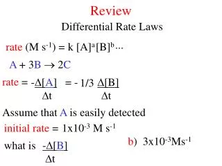
Review Differential Rate Laws ... rate (M s-1) = k [A]a [B]b A + 3B 2C rate = -[A] t = - [B] t 1/3 Assume that A is easily detected initial rate = 1x10⁻³ M s-1 a) 1x10⁻³Ms-1 b) 3x10⁻³Ms-1 c) 0.33x10⁻³Ms-1 -[B] t what is
[A] [A] Concentration (M) Concentration (M) t (ms) t (ms) Exp. 1 [B]i initial rate [A]i (M) (M) (M s-1) 1.0 1.0 1.0 x 10⁻³ Exp. 2 [A]i [B]I initial rate (M)(M)(M s-1) 2.0 1.0 2.0 x 10⁻³ Exp. 3 [A]i [B]I initial rate (M)(M)(M s-1) 1.0 x 10⁻³ 1.0 2.0
Exp. 1 k rate = [A]a [B]b [A]i [B]I initial rate (M)(M)(M s-1) 1.0 1.0 a = 0 a = 1 a = 2 2 x 10-3 = 1 x 10⁻³ [2.0]a [1.0]a rate 2 = rate 1 1.0 x 10⁻³ Exp. 2 1 x 10-3 = 1 x 10⁻³ rate 3 = rate 1 [2.0]b [1.0]b b = 0 b = 1 b = 2 [A]i [B]I initial rate (M)(M)(M s-1) 2.0 1.0 rate = k [A] 2.0 x 10⁻³ 1storder reaction Exp. 3 [A]i [B]I initial rate (M)(M)(M s-1) 1.0 2.0 1x10⁻³(M s-1) = k [1.0 M] k = 1 x 10⁻³ s-1 1.0 x 10⁻³
Concentration (M) t (ms) Exp [A]i [B]i initial rate (M) (M) (M s-1) 1 1.0 1.0 1.0 x 10⁻³ 2 2.0 1.0 2.0 x 10⁻³ 3 1.0 2.0 2.0 x 10⁻³ 4 2.02.0 4.0 x 10⁻³ 2.0 x 10-3 = 1.0 x 10⁻³ rate 2 = rate 1 [2.0]a [1.0]a 1st order in [A] a = 1 2.0 x 10-3 = 1.0 x 10⁻³ rate 3 = rate 1 [2.0]b [1.0]b 1st order in [B] b = 1 rate = k [A] [B] 2nd order reaction
ln Integrated rate laws differential rate laws are differential equations t = t rate = k[A] = -d[A]/dt t = 0 rate = k[A]2 = -d[A]/dt differential rate eqn integrated rate eqn rate = k[A] [A]t = - kt [A]0
ln [A]t = - kt [A]0 Integrated rate laws ln[A]t = ln[A]t - ln[A]0 -kt + ln[A]0 = - kt y = mx + b y = ln[A]t x = t m = -k b = ln[A]0 ln[A]t plot v.s. t linear
[A] Concentration (M) t (ms) ln [A] ln [A] rate = k[A] ln[A]t = - kt + ln[A]0 y = ln[A]t x = t m = -k b = ln[A]0
ln [A]t = - kt [A]0 ln 1st order reactions ln[A]t = - kt + ln[A]0 2N2O5(g) 4NO2(g) + O2(g) rate = (M s-1) k [N2O5 ] (M) k = 5.1 x 10⁻⁴ s-1 What is [N2O5] after 3.2 min if [N2O5] = 0.25M 0 [N2O5] = - (5.1x10⁻⁴s-1) (192 s) 3.2 [0.25] [N2O5]3.2 = 0.23 M
ln 1st order reactions ln [A]t = - kt [A]0 ln[A]t = - kt + ln[A]0 How long will it take for [N2O5] to go from 0.25 M to 0.125 M ? [0.125] = t = 23 min - (5.1x10⁻⁴s-1) t [0.25] The half-life (t1/2) is the time required for [reactant] to decrease to 1/2 [reactant]i t1/2= ln 2 k
1st order reactions t1/2=ln 2 k 700 ms = ln 2 k k 1 s-1 Radioactive decay 1st order 14C dating t1/2 = 5730 years
1 1 [A]0 [A]t Integrated rate laws differential rate eqn integrated rate eqn ________________________ ________________________ rate = k[A] ln [A]t = - kt [A]0 1st order = kt + rate = k[A]2 2nd order y = mx + b y = 1 [A]t x = t m = k b = 1 [A]0 A plot of v.s. is linear 1/[A]t t
[A] rate = k[A]2 t1/2 = 1 k[A]0 1 = kt + 1 [A]t [A]0 1/[A]
Integrated rate laws second order reactions rate = k [A]2 1 = kt + 1 [A]t [A]0 many second order reactions rate = k [A] [B] A + B C A and B consumed stoichiometrically [A]0 = [B]0 if not, no analytical solution
Pseudo 1st order reactions high order reactions difficult to analyze put in large excess of all but one reagent [A]0 [B]0 rate =k [A]a [B]b 1.0 x 10⁻³ M 1.0 M [B] constant -0.5 x 10⁻³ mol -0.5x 10⁻³ mol rate = k’ [A]a 0.5 x 10⁻³ M 0.999 M k = k’ k[A]a[B]b = k’[A] [B]b


