Optimizing Inventory Management with EOQ and R for Air Filters: A Case Study
This case study explores an inventory management optimization scenario for air filters, focusing on the Economic Order Quantity (EOQ) and Reorder Point (R). With an annual purchase rate of 800 units, order costs of $10, and a unit cost of $25 per filter, we analyze the impact of carrying costs and shortage costs, along with demand variations. Through iterative calculations based on demand distributions and lead times, we derive optimal inventory strategies, ultimately achieving convergence on (Q*, R*) values. Key insights into demand patterns inform effective inventory control.

Optimizing Inventory Management with EOQ and R for Air Filters: A Case Study
E N D
Presentation Transcript
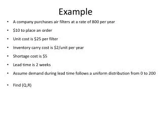
Example • A company purchases air filters at a rate of 800 per year • $10 to place an order • Unit cost is $25 per filter • Inventory carry cost is $2/unit per year • Shortage cost is $5 • Lead time is 2 weeks • Assume demand during lead time follows a uniform distribution from 0 to 200 • Find (Q,R)
Solution • Partial derivative outcomes:
Solution • From Uniform U(0,200) distribution:
0 200 R Solution • Iteration 1: F(R)
Solution • Iteration 2:
Solution • Iteration 3:
Solution • R didn’t change => CONVERGENCE • (Q*,R*) = (94,190) I(t) 253 Slope -800 190 159 With lead time equal to 2 weeks: SS = R – lt =190-800(2/52)=159
Example • Demand is Normally distributed with mean of 40 per week and a weekly variance of 8 • The ordering cost is $50 • Lead time is two weeks • Shortages cost an estimated $5 per unit short to expedite orders to appease customers • The holding cost is $0.0225 per week • Find (Q,R)
Solution • Demand is per week. • Lead time is two weeks long. Thus, during the lead time: • Mean demand is 2(40) = 80 • Variance is (2*8) = 16 • Demand observed in one week is independent from demand observed in any other week: • E(demand over 2 weeks) = E (2*demand over week 1) = 2 E(demand in a single week) = 2 μ = 80 Standard deviation over 2 weeks is σ = (2*8)0.5 = 4
Finding Q and R, iteratively • 1. Compute Q = EOQ. • 2. Substitute Q in to Equation (2) and compute R. • Use R to compute average backorder level, n(R) to use in Equation (1). • 4. Solve for Q using Equation (1). • 5. Go to Step 2 until convergence.
Solution • Iteration 1: • From the standard normal table:
Solution • Iteration 2: This is the unit normal loss expression. Table A - 4 gives values.
Solution • Iteration 2: