Download

1 / 29
290 likes | 419 Views
Discrete Fourier Transform and Applied Spectral Analysis. у. у. (1.11). Correlation Functions. Stationary Random processes. Cross Correlation Functions. From obvious expression:. It could be derived:. Ergodic Random Processes. Power Spectral Densities of the Ergodic Random Processes.

E N D
у у (1.11) Correlation Functions
Stationary Random processes Cross Correlation Functions From obvious expression: It could be derived:
Ergodic Random Processes Power Spectral Densities of the Ergodic Random Processes
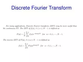
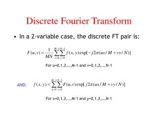
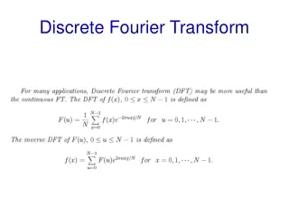
Discrete Fourier transform Let - periodicity interval of continuous function -the lowest frequency , then: ,where m - integer number. Fourier series: (1) Coefficients: (2) Continuous Fourier transform: Direct: (3) (4) Inverse:
The lowest frequency and increment of the angular frequency Direct Discrete Fourier transform (DFT): Current frequency “k” is the time domain index, “n” is the frequency domain index Relative frequency: Inverse Discrete Fourier transform (IDFT):
(10) Direct DFT: Inverse DFT : Properties of DFT: 1) symmetry property 2) skew-symmetry of the algorithm (11) (12)
Computation of DFT and IDFT. When k=N, Presentation of DFT in the form of IDFT:
FFT and IFFTAlgorithms If (1) Then (2) or (3) z(k) and y(k) are samples of the process in the time domain.
Then (1) can be rewritten as: (4) or N dimension In order to save memory cells, it is possible to save Y(n) and Z(n) in the same register: (5) 1 array of N dimension is transformed in (3) where (6)
1 1 - - - - Taking into account: We receive: (7) “Butterfly” graph (algorithm)
1 + - Example: transformation of two 4-points DFT in one 8-points DFT Example: Transformation of 2- and 4-pointed ДПФ in the 8-pointed one Common representation in graph form:
Transition from N/4-points to N/2-points DFT: Small Turn Factor
Transition from 2-points to 4-points DFT: Adjacency matrix
Power Spectral Density estimation Power or variance: Power Spectral Density:
Periodogram: Convolution in the Frequency Domain: -time domain: -frequency domain:
x(t) 2 1 t T -T Gibbs Phenomenon |X (T)| =|sinc(T)| X(T)=sinc(T)
Frequency Domain Representation of the Rectangular Window in the Logarithmic Scale
(3) GeneralizedHann –Hemming Window Blackman Window (4) (4) Flat Top Window (5)
(6) Kaiser Window
Spectral Resolution: (7) Bias of the Periodogram: (8) Variance of the Periodogram: (9)
Parseval's theorem: Estimations of cross spectra (10) (11) (12) (13) (14) The square of coherence coefficient: (15) (16) (17)
Error variances (18) Stochastic process generation. Rice-Pearson decomposition. (19) (20) (21)
References • MATLAB: “Signal Processing Toolbox. User’s Guide”.Math Works, 2011.-363 p. • В.П. Бабак, В.С. Хандецький, Е. Шрюфер. Обробка сигналів. Київ, «Либідь», 1999.- 495с.