Download
1 / 37
390 likes | 664 Views
ECSE-4963 Introduction to Subsurface Sensing and Imaging Systems. Lecture 2: Introduction to MATLAB Kai Thomenius 1 & Badri Roysam 2 1 Chief Technologist, Imaging technologies, General Electric Global Research Center 2 Professor, Rensselaer Polytechnic Institute.

E N D
ECSE-4963Introduction to Subsurface Sensing and Imaging Systems Lecture 2: Introduction to MATLAB Kai Thomenius1 & Badri Roysam2 1Chief Technologist, Imaging technologies, General Electric Global Research Center 2Professor, Rensselaer Polytechnic Institute Center for Sub-Surface Imaging & Sensing
Review of Last Lecture • Subsurface imaging – Course Focus • Many applications to Biology, Medicine, Industry, & Homeland Security • Probes, media, and probe-media interactions • Methods by which we examine contents of hidden volumes • Wave theory the common thread • Common to electromagnetic and acoustic probing • This Class: • Overview of Matlab tools
THE BIG PICTURE What is subsurface sensing & imaging? Why a course on this topic? EXAMPLE: THROUGH TRANSMISSION SENSING X-Ray Imaging Computer Tomography COMMON FUNDAMENTALS propagation of waves interaction of waves with targets of interest PULSE ECHO METHODS Examples MRI A different sensing modality from the others Basics of MRI MOLECULAR IMAGING What is it? PET & Radionuclide Imaging IMAGE PROCESSING & CAD Outline of Course Topics
Matlab in this Course • Some of the imaging modalities we will study have well established Matlab-based simulations. • We will reconstruct CT, ultrasound, and possibly optical images with Matlab. • We will also model acoustic fields with Matlab.
Sources • These slides have been collected from a number of sources: • www.cs.cornell.edu/Courses/cs401/2001fa • www.soes.soton.ac.uk/MSc/current/matlab.ppt • Matlab File Exchange • www.mathworks.com/matlabcentral/fileexchange/loadCategory.do • While there, download the following: MATLAB Programming Style Guidelines by Richard Johnson
Matlab History Matlab stands for “Matrix Laboratory” Created by Dr. Cleve Moler in the 1970s, then a professor at U. of New Mexico Now Dr. Moler is Chief Scientist Mathworks, Inc. Mathworks is now a major computer company Developed from LAPACK--a series of routines for numerical linear algebra Consequences: * is funny, / is even funnier Matlab does linear algebra really well
Starting Up • On Windows: • Launch from START, or find matlab.exe & double click • On UNIX/Linux • Open a terminal, type “matlab” • Problems: • “Command not found”--check your path • Splash window of 6.X hangs--try “matlab -nojvm”
Matlab Windows • As of 6.0, Matlab has lots of windows inside a “Desktop” • The Workspace is the center of the Matlab universe • Holds your data • Waits for your commands • (other windows are fluff) • 5.X only has workspace
Basic Math Matlab is a command-line calculator Simple arithmetic operators + - * / ^ Basic functions sin(), log(), log10(), exp(), rem() Constants pi, e
Big deal, a calculator’s $2 Matlab is a fully-functional programming language This means we get variables name = value Name can be anything made of letters, numbers, and a few symbols (_). Must start with a letter End line with “;” to avoid output Can also use “;” to put multiple commands on a line List with who Delete with clear More info with whos
1D Arrays—a.k.a. Vectors An array is anything you access with a subscript 1D arrays are also known as “vectors” Everything (nearly) in Matlab is a “double array” Create arrays with brackets [ ] Separate elements with commas or spaces Access with ()’s
Regular arrays We can create regularly spaced arrays using “:” A=st:en produces [st, st+1, st+2, … en] A=1:5 is [1 2 3 4 5] A=-3.5:2 is [-3.5 -2.5 -1.5 0.5 1.5]---note, stops before 2! What happens if en < st ? Can also insert a “step” size: A=st:step:en A=0:2:6 is [0 2 4 6] A=5:-2.5:0 is [5 -2.5 0];
Accessing vectors Matlab arrays start at 1 In most languages (C, Java, F77) can only access arrays one element at a time: a(1)=1; a(2)=2.5; a(3)=-3; etc. In Matlab, can access several elements at a time using an array of integers (aka an index) a(1:5) is [a(1),a(2),a(3),a(4),a(5)] a(5:-2:1) is [a(5), a(3), a(1)]
Accessing vectors Index vectors can be variables: A=10:10:100; I=[1:2:9]; A(I) gives [10,30,50,70,90] J=[2:2:10];A(J) gives [20,40,60,80,100]; What does A(I)=A(J) do?
Column vectors “row vectors” are 1-by-n “column vectors” are n-by-1 Row/column distinction doesn’t exist in most languages, but VERY IMPORTANT in MATLAB Create column vectors with semi-colons Can force to column vector with (:) Convert column-to-row and back with transpose (’) Can access the same way as row vectors
2D arrays--matrices From using commas/spaces and semi-colons A=[1 2 3; 4 5 6; 7 8 9]; A(j,k)= j’th row, k’th column A(2:3,1:2)= rows 2 through 3 and columns 1 through 2 A([1,3,4], :)= all of rows 1, 3 and 4 A(:, 1)= first column
“A is m-by-n” means A has m rows and n columns [m,n]=size(A) gets size of A length(a) gets length of vectors. A(1:3,2)=v, v better have length 3 A(1:2:5,2:3)=B, B better be 3-by-2 Size matters
Array Arithmetic C=A+B if A and B are the same size, C(j,k)=A(j,k)+B(j,k) If A is a scalar, C(j,k)=A+B(j,k) Same for -
Array Multiplication Multiplication is weird in Matlab Inherited from linear algebra To multiply by a scalar, use * To get C(j,k)=A(j,k)*B(j,k) use “.*” Also applies to “.^” and “./”
Matrix Multiplication C=A*B A is m-by-p and B is p-by-n then C is m-by-n: C(i,j)= a(i,1)*b(1,j)+a(i,2)*b(2,j)+ … + a(i,p)*b(p,j) Another view: C(i,j)=a(i,:)*b(:,j); 1-by-p p-by-1 answer is 1-by-1
ND arrays Until V5, Matlab arrays could only be 2D Now has unlimited dimensions: A=ones(2,3,2) A is a 3D array of ones, with 2 rows, 3 columns, and 2 layers A(:,:,1) is a 2-by-3 matrix squeeze command is very important
What kind of graphics is possible in Matlab? Polar plot: t=0:.01:2*pi; polar(t,abs(sin(2*t).*cos(2*t))); Line plot: x=0:0.05:5;,y=sin(x.^2);,plot(x,y); Stem plot: x = 0:0.1:4;, y = sin(x.^2).*exp(-x); stem(x,y)
What kind of graphics is possible in Matlab? Surface plot: z=peaks(25);, surf(z);, colormap(jet); Mesh plot: z=peaks(25);, mesh(z); Contour plot: z=peaks(25);,contour(z,16); Quiver plot: 28 January 2003, Matlab tutorial: Joanna Waniek (jowa@soc.soton.ac.uk)
Iteration For loops in Matlab use index-notation: for j=st:step:en; <commands involving j> ; end Example: u’*v tot=0; for j=1:length(u); tot=tot+u(j)*v(j); end
Conditionals Conditional statements control flow of a program if(logic); <commands executed if true>; else; <commands executed if false>; end Matlab also has switch: switch(j); case a: <commands if a=j>; case b: <commands if b=j>; … otherwise: <default commands>; end
Find--searches for the truth (or not false) b=[1 0 -1 0 0]; I=find(b) I=1 3 --b(I) is an array without zeros I=find(ones(3,1)*[ 1 2 3]==2) I= 4 5 6 [I,J]=find(ones(3,1)*[ 1 2 3]==2) I= 1 2 3 J= 2 2 2 Logic--searching with find
Programming • Matlab programs are stored in “m-files” • Text files containing Matlab commands and ending with .m • Script m-files--commands executed as if entered on command line • Function m-files--analogous to subroutines or methods, maintain their own memory (workspace)
Functions First line of file must be function [outputs]=fname(inputs) outputs and inputs can be blank Comments immediately following are returned by help Functions must be in current directory or in Matlab’s search path
Image data 2D image Matrix of “point” measurements Point = pixel Size: ∆x, ∆y Non-isotropic images: ∆x ≠ ∆y Dynamic range = 2N 3D image Point = voxel Axial extent = ∆z Image sequence (movie) of living systems Time sequence of 2D/3D images Temporal interval = ∆t Multi-spectral / multi-channel image Each pixel/voxel is vector valued Each element = spectral band (λ) or “channel” Special case: color RGB images Multi-modal image Each pixel/voxel is vector valued Each element corresponds to an imaging modality Pixel intensity: Represents value of a physical property of the tissue at that point
Dealing with Image Data • The MATLAB Image Processing toolbox is part of the RPI installation package • Provides functions for reading, visualizing, transforming, and analyzing images, and image sequences (video) • The coordinate system for images is a bit quirky • Need to transform real-valued matrices X to an image format using the function I = mat2gray(X) before displaying it, and vice versa • A = imread(filename) will read an image in most common formats • imshow(I) will display an image • Contains functions for doing some image reconstruction (e.g., x-ray tomography) • Work through Chapters 1 & 2 of Image Processing Toolbox manual to become familiar with grayscale and color images, and commands for converting matrices to images and vice versa • PDF online on mathworks.com
Color Maps and Color Images • A point on the screen is usually a triplet of 3 numbers [red, green, blue] or RGB • True color images have 3 bytes/pixel • An indexed image has a color map • Maps a brightness I to an RGB value • Much more compact • We can display grayscale images (one channel) using a color map as a pseudo color image • Many color maps available in MATLAB • Conversion routines: • Gray2 ind, ind2gray, rgb2gray, mat2gray, etc index
Image Tool is Handy • Allows you to view images, pixel values, overall image characteristics, magnify, shrink, crop, measure distances, adjust contrast, brightness, etc.
Matlab Alternatives • While it has become a standard, MATLAB has garnered a set of critics. • Part of this is due to the cost – very expensive for companies. • Some open source alternatives: • Octave • FreeMat (nearly identical syntax to Matlab) • SciLab • There is a version that runs under the Palm OS called Lyme.
Summary • MATLAB • Very widely used mathematical modeling tool • Brief introduction to MATLAB’s key concepts • Arrays, vectors, matrices, their addressing • Graphics w. MATLAB • Iteration & program flow • Conditionals • Image Processing Toolbox is very useful for this course • Make sure to download the PDF online manual (very helpful!) • Other toolkits include Statistics, Control, etc. • Important Advice: • ALWAYS check the online manual page for any new MATLAB function before using it • ALWAYS try out the example on the manual page first, and then adapt/modify it to your needs. • Next Class: • Projection Imaging – X-rays
Instructor Contact Information Badri Roysam Professor of Electrical, Computer, & Systems Engineering Office: JEC 7010 Rensselaer Polytechnic Institute 110, 8th Street, Troy, New York 12180 Phone: (518) 276-8067 Fax: (518) 276-6261/2433 Email: roysam@ecse.rpi.edu Website: http://www.ecse.rpi.edu/~roysabm Secretary: Laraine Michaelides, JEC 7012, (518) 276 –8525, michal@rpi.edu
Instructor Contact Information Kai E Thomenius Chief Technologist, Ultrasound & Biomedical Office: KW-C300A GE Global Research Imaging Technologies Niskayuna, New York 12309 Phone: (518) 387-7233 Fax: (518) 387-6170 Email: thomeniu@crd.ge.com, thomenius@ecse.rpi.edu Secretary: TBD