Download

1 / 29
290 likes | 418 Views
This paper introduces the Intensity Gamma approach for pricing collateralized debt obligations (CDOs) and explores its advantages over traditional models. Drawing inspiration from the Variance Gamma model, it emphasizes inducing correlation through business time instead of calendar time. The authors present a detailed calibration method for constructing survival curves and default intensity paths, offering insights into pricing non-standard tranches and exotic credit derivatives. Through rigorous testing, the method showcases improved accuracy and a practical framework for financial professionals.

E N D
Pricing CDOs using Intensity Gamma Approach Christelle Ho Hio Hen Aaron Ipsa Aloke Mukherjee Dharmanshu Shah
Intensity Gamma • M.S. Joshi, A.M. Stacey “Intensity Gamma: a new approach to pricing portfolio credit derivatives”, Risk Magazine, July 2006 • Partly inspired by Variance Gamma • Induce correlation via business time
Business time Calendar time Business time vs. Calendar time
Calibration Parameter guess Survival Curve Construction 6mo 1y 2y .. 5y name1 . name2 . . name125 IG Default Intensities CDS spreads Tranche pricer Default time calculator Business time path generator 0-3% … 3-6% … 6-9% … . . Market tranche quotes Objective function NO Err<tol? YES Block diagram
Advantages of Intensity Gamma • Market does not believe in the Gaussian Copula • Pricing non-standard CDO tranches • Pricing exotic credit derivatives • Time homogeneity
The Survival Curve • Curve of probability of survival vs time • Jump to default = Poisson process P(λ) • Default = Cox process C(λ(t)) • Pr (τ > T) = exp[ ] • Intensity vs time – λT1, λT2, λT3….. for (0,T1), (0,T2), (0,T3)
Bootstrapping the Survival Curve • Assume a value for λT1 • X(0,T1) = exp(-λT1 . T1) • Price CDS of maturity T1 • Use a root solving method to find λT1 • Assume a value for λT2 • Now X(0,T2) = X(0,T1) * exp(-λT2(T2-T1)) • Price CDS of maturity T2 • Use root solving method to find λT2 • Keep going on with T3, T4….
Constructing a Business Time Path • Business time modeled as two Gamma Processes and a drift.
Constructing a Business Time Path • Characteristics of the Gamma Process • Positive, increasing, pure jump • Independent increments are Gamma distributed:
Constructing a Business Time Path • Series Representation of a Gamma Process (Cont and Tankov) • T,V are Exp(1), No Gamma R.V’s Req’d.
Constructing a Business Time Path Truncation Error Adjustment
Constructing a Business Time Path Truncation Error Adjustment
Constructing a Business Time Path • Test Effect of Estimating Truncation Error in Generating 100,000 Gamma Paths • 1. Set Error = .001, no adjustment • Computation Time = 42 Seconds • 2. Set Error = 0.05 and apply adjustment • Computation Time = 34 seconds
Constructing a Business Time Path • Testing Business Time Paths • Given drift a = 1, Tenor = 5, 100,000 paths Mean = 63.267 +/- 0.072 Expected Mean = 63.333
Constructing a Business Time Path …Testing Business Time Path Continued Variance = 522.3 Expected Variance = 527.8
IG Forward Intensities ci(t) • In IG model survival probability decays with business time • Inner calibration: parallel bisection • Note that one parameter redundant
Default Times from Business Time • Survival Probability: • Default Time:
Tranche pricer • Calculate cashflows resulting from defaults • Validation: reprice CDS (N=1) EDU>> roundtriptest(100,100000); closed form vfix = 0.0421812, vflt = 0.0421812 Gaussian vfix = 0.0422499, vflt = 0.0428865 IG vfix = 0.0429348, vflt = 0.0422907 input spread = 100, gaussian spread = 101.507, IG spread = 98.4998 • Validation: recover survival curve
A Fast Approximate IG Pricer • Constant default intensities λi • Probability of k defaults given business time IT • Price floating and fixed legs by integrating over distribution of IT
Fast IG Approximation Comparison Tranche Fast IG Full IG 0-3% 1429 1778 3-7% 135 187 7-10% 14 29 10-15% 1 5 15-30% 0 0
Fast Approx – Both Constant λi Tranche Fast IG Full IG 0-3% 1429 1573 3-7% 135 133 7-10% 14 13 10-15% 1 1 15-30% 0 0
Fast Approx – Const λi, Uniform Default Times Tranche Fast IG Full IG 0-3% 1584 1573 3-7% 144 133 7-10% 14 13 10-15% 1 1 15-30% 0 0
Calibration • Unstable results => need for noisy optimization algorithm. • Unknown scale of calibration parameters => large search space. • Long computation time => forbids Genetic Algorithm Simulated Annealing
Calibration • Redundant drift value => set a = 1 • Two Gamma processes: = 0.2951 = 0.2838 = 0.0287 = 0.003
Future Work • Performance improvements • Use “Fast IG” as Control Variate • Quasi-random numbers • Not recommended for pricing different maturities than calibrating instruments • Stochastic delay to default • Business time factor models